<?xml version="1.0" encoding="utf-8"?><feed xmlns="http://www.w3.org/2005/Atom" ><generator uri="https://jekyllrb.com/" version="3.10.0">Jekyll</generator><link href="https://blog.kyoseung.me/feed.xml" rel="self" type="application/atom+xml" /><link href="https://blog.kyoseung.me/" rel="alternate" type="text/html" /><updated>2026-08-24T11:55:04+00:00</updated><id>https://blog.kyoseung.me/feed.xml</id><title type="html">Database stuff</title><subtitle>related to database</subtitle><author><name>Kyoseung Koo</name><email>grammaright@gmail.com</email></author><entry><title type="html">NoSQL 개요: 등장 배경, CAP/BASE, 그리고 대표적 데이터 모델</title><link href="https://blog.kyoseung.me/nosql/2025/08/31/nosql-basic-concepts-and-theory-ko.html" rel="alternate" type="text/html" title="NoSQL 개요: 등장 배경, CAP/BASE, 그리고 대표적 데이터 모델" /><published>2025-08-31T09:00:00+00:00</published><updated>2025-08-31T09:00:00+00:00</updated><id>https://blog.kyoseung.me/nosql/2025/08/31/nosql-basic-concepts-and-theory-ko</id><content type="html" xml:base="https://blog.kyoseung.me/nosql/2025/08/31/nosql-basic-concepts-and-theory-ko.html"><![CDATA[<p><em>이 글은 제가 2025년 8월 31일에 진행한 “NoSQL 기본 개념 및 이론” 세미나 내용을 기반으로 작성되었습니다.</em></p>

<hr />

<h2 id="nosql의-정의-및-등장-배경">NoSQL의 정의 및 등장 배경</h2>
<p><strong>NoSQL</strong>은 ‘Not only SQL’의 줄임말로, 관계형 데이터베이스(RDBMS)가 아닌 다른 데이터 모델 기반의 데이터베이스 시스템을 사용하는 <strong>움직임</strong>입니다. NoSQL은 RDBMS가 가진 엄격한 스키마 및 <strong>ACID(Atomicity, Consistency, Isolation, Durability)</strong> 트랜잭션 모델의 한계를 극복하기 위해 등장했습니다.</p>

<p>웹, 모바일, 사물 인터넷(IoT) 기기 등으로부터 발생하는 데이터의 양과 속도가 폭발적으로 증가하고 있습니다. 이러한 데이터의 특성은 <strong>빅데이터의 3V</strong>로 요약할 수 있습니다.</p>

<ul>
  <li><strong>Volume (규모)</strong>: 처리해야 할 데이터의 양이 굉장히 크게 증가했습니다.</li>
  <li><strong>Velocity (속도)</strong>: 데이터가 생성되고 소비되는 속도가 매우 빨라졌습니다.</li>
  <li><strong>Variety (다양성)</strong>: 데이터의 형태가 정형 데이터뿐만 아니라 반정형 및 비정형 데이터까지 포함하며 다양해졌습니다.</li>
</ul>

<p>전통적인 RDBMS는 이러한 3V의 특성을 처리하는 데 있어 여러 한계에 직면합니다.</p>

<ul>
  <li><strong>Volume &amp; Velocity</strong>: 전통적인 RDBMS는 엄격한 ACID 트랜잭션 모델 때문에 데이터 분산 및 처리에 오버헤드가 발생합니다. 이로 인해 수평적 확장이 어렵고, 빠르게 생성되는 대용량의 데이터를 처리하는 데 한계가 나타납니다.</li>
  <li><strong>Variety</strong>: RDBMS는 고정된 스키마를 요구하므로, 형태가 일정하지 않은 비정형 또는 반정형 데이터를 저장하기 어렵습니다.</li>
</ul>

<h2 id="nosql의-일반적인-특징">NoSQL의 일반적인 특징</h2>
<p>NoSQL 시스템은 RDBMS와 구분되는 몇 가지 공통적인 특징을 가집니다.</p>
<ul>
  <li><strong>유연한 스키마</strong>: 엄격한 스키마 없이 데이터를 저장할 수 있어 다양한 형태의 데이터 관리에 용이합니다.</li>
  <li><strong>어그리게이션 지향(Aggregation oriented)</strong>: RDBMS의 정규화(Normalization)와 달리, 관련 데이터를 하나의 단위로 묶어 저장하여 데이터 접근을 단순화합니다. 이는 비정규화(de-normalization)된 형태로 데이터를 관리하는 것을 의미합니다.</li>
  <li><strong>약한 일관성 모델</strong>: RDBMS의 <strong>ACID</strong>와 달리, <strong>BASE</strong>라는 일관성 모델을 따릅니다. 이는 강력한 일관성을 일부 완화하여 높은 가용성(high availability)과 낮은 지연 시간(low latency)을 확보합니다.</li>
  <li><strong>분산 처리 친화성</strong>: NoSQL은 처음부터 분산 환경에 최적화되어 설계되었기 때문에 여러 서버에 데이터를 분산하여 저장하고 처리하는 데 있어 훨씬 효율적입니다. 이로 인해 대규모 환경에서 수평적 확장이 용이합니다.</li>
</ul>

<h2 id="nosql의-주요-이론-cap-및-base">NoSQL의 주요 이론: CAP 및 BASE</h2>

<p>NoSQL의 약한 일관성 모델을 이해하기 위해서는 <strong>CAP 정리</strong>를 먼저 살펴봐야 합니다. CAP은 2000년 Eric Brewer가 <strong>CAP Conjecture</strong>라는 가설로 제안하였으며, 이후 2002년 Seth Gilbert와 Nancy Lynch에 의해 증명되었습니다. 이 이론은 분산 시스템이 <strong>일관성(Consistency)</strong>, <strong>가용성(Availability)</strong>, <strong>분할 내성(Partition tolerance)</strong> 중 최대 두 가지만을 동시에 만족할 수 있다는 것을 설명합니다.</p>

<ul>
  <li><strong>일관성(Consistency)</strong>: 모든 클라이언트가 어느 노드에 접근하든 동일한 최신 데이터에 접근할 수 있도록 보장합니다.</li>
  <li><strong>가용성(Availability)</strong>: 시스템의 모든 노드가 요청에 대해 항상 응답할 수 있도록 보장합니다.</li>
  <li><strong>분할 내성(Partition tolerance)</strong>: 네트워크 분할(노드 간 통신 단절)과 같은 장애 상황에서도 시스템이 정상적으로 동작하는 것을 보장합니다.</li>
</ul>

<p>NoSQL은 일반적으로 <strong>가용성</strong>과 <strong>분할 내성</strong>을 선택하고, <strong>일관성</strong>을 일부 희생하는 경향을 보입니다. 많은 NoSQL 시스템이 채택하는 <strong>BASE</strong> 모델은 이러한 가용성 중시의 결과입니다.</p>

<ul>
  <li><strong>Basically Available</strong>: 시스템의 모든 노드가 데이터를 처리할 수 있도록 보장합니다. 노드 장애가 발생해도 시스템은 지속적으로 동작합니다.</li>
  <li><strong>Soft state</strong>: 데이터의 상태는 트랜잭션 종료 후에도 즉각적으로 일관되지 않을 수 있으며, 이는 입력이 없어도 시스템의 상태가 변할 수 있다는 의미를 포함합니다. 데이터의 최종적인 상태는 일정 시간이 지나야 확정됩니다.</li>
  <li><strong>Eventually consistent</strong>: 모든 노드에 데이터 업데이트가 전파되면, 최종적으로 모든 노드가 동일한 데이터를 갖게 됩니다. 이러한 일관성은 즉각적이지 않고 시간이 걸립니다.</li>
</ul>

<h2 id="주요-nosql-데이터-저장소">주요 NoSQL 데이터 저장소</h2>

<p>NoSQL은 저장하는 데이터의 형태에 따라 크게 네 가지로 분류됩니다. 이 섹션에서는 각 데이터 저장소의 특징과 대표적인 예시를 설명합니다.</p>

<h3 id="키-값-저장소key-value-stores">키-값 저장소(Key-value stores)</h3>

<p>키-값 저장소는 데이터를 고유한 <strong>키(Key)</strong>와 이에 연결된 <strong>값(Value)</strong>의 쌍으로 저장합니다. 이는 가장 단순한 형태의 데이터 모델로, 매우 빠른 읽기 및 쓰기 성능을 제공합니다. 값의 형태에는 제약이 없으므로, 문자열, JSON 객체, 이미지, 파일 등 다양한 데이터를 저장할 수 있습니다. 이러한 단순성 덕분에 <strong>Redis, RocksDB, AWS DynamoDB</strong>와 같은 시스템에 널리 활용됩니다. 대부분의 키-값 저장소는 내부적으로 <strong>LSM-Tree(Log-Structured Merge-Tree)</strong>를 사용하여 쓰기 성능을 최적화합니다.</p>

<h3 id="와이드-컬럼-저장소wide-column-stores">와이드-컬럼 저장소(Wide-column stores)</h3>

<p>와이드-컬럼 저장소는 RDBMS가 사용하는 테이블 구조와 같은 방식으로 데이터를 구성하지만, 스키마에 컬럼이 미리 정의되지 않아도 동적으로 컬럼을 추가할 수 있습니다.
즉, 각 행이 서로 다른 컬럼 집합을 가질 수 있습니다.
이는 스파스(sparse) 데이터를 관리하는 데 유리합니다. 
 <strong>Apache Cassandra와 HBase</strong>가 대표적인 예시이며, 대규모 로그 데이터나 시계열 데이터와 같이 행마다 열이 다양하게 추가되는 환경에 적합합니다. 대부분의 와이드-컬럼 저장소는 키-값 저장소를 스토리지 엔진으로 사용합니다.</p>

<h3 id="문서-저장소document-stores">문서 저장소(Document stores)</h3>

<p>문서 저장소는 데이터를 <strong>문서(Document)</strong> 형태로 저장합니다. 이 문서는 일반적으로 JSON과 같은 반정형 데이터 형식을 따릅니다. 
문서 내의 값으로 다시 중첩된 문서(nested-document)가 들어갈 수 있어 전체적으로 <strong>트리(Tree)</strong> 형태의 계층 구조를 가집니다.
문서 저장소는 고정된 스키마가 필요 없어 구조가 다른 데이터를 동일한 컬렉션에 저장할 수 있으므로, RDBMS의 고정된 테이블 구조보다 훨씬 유연합니다.
<strong>MongoDB와 Couchbase</strong>가 널리 사용됩니다.
MongoDB는 내부적으로 <strong>WiredTiger</strong>라는 스토리지 엔진을 사용합니다. 이 엔진은 데이터를 저장할 때 JSON과 유사한 이진 포맷인 <strong>BSON</strong>을 사용하여 효율적으로 문서를 관리합니다.</p>

<h3 id="그래프-저장소graph-stores">그래프 저장소(Graph stores)</h3>

<p>그래프 저장소는 데이터 엔티티를 나타내는 <strong>정점(Vertex)</strong>과 그들 간의 관계인 <strong>간선(Edge)</strong>으로 표현되는 그래프 데이터를 저장하는 데 사용됩니다.
이러한 구조는 복잡한 관계를 효율적으로 탐색하는 데 강점을 가지며, 소셜 네트워크, 추천 시스템, 지식 그래프 등에 활용됩니다.
<strong>Neo4j</strong>가 대표적인 예시이며, Neo4j는 <strong>index-free adjacency</strong>라는 스토리지를 사용해 데이터 노드와 관계를 직접적인 포인터로 연결하여 빠른 탐색 속도를 보장합니다.</p>

<h2 id="결론">결론</h2>

<p>이 글에서는 NoSQL의 정의, 등장 배경, 일반적인 특징, 그리고 주요 데이터 모델에 대해 개괄적으로 살펴보았습니다. 다음 글부터는 각 모델 별 저장소의 <strong>스토리지 엔진</strong>에 대해 더 깊이 있게 논의할 예정입니다.</p>]]></content><author><name>Kyoseung Koo</name><email>grammaright@gmail.com</email></author><category term="nosql" /><summary type="html"><![CDATA[이 글은 제가 2025년 8월 31일에 진행한 “NoSQL 기본 개념 및 이론” 세미나 내용을 기반으로 작성되었습니다.]]></summary></entry><entry><title type="html">NoSQL Overview: Background, CAP/BASE, and Representative Data Models</title><link href="https://blog.kyoseung.me/nosql/2025/08/31/nosql-basic-concepts-and-theory.html" rel="alternate" type="text/html" title="NoSQL Overview: Background, CAP/BASE, and Representative Data Models" /><published>2025-08-31T09:00:00+00:00</published><updated>2025-08-31T09:00:00+00:00</updated><id>https://blog.kyoseung.me/nosql/2025/08/31/nosql-basic-concepts-and-theory</id><content type="html" xml:base="https://blog.kyoseung.me/nosql/2025/08/31/nosql-basic-concepts-and-theory.html"><![CDATA[<p><em>This post is a translated version of <a href="/nosql/2025/08/31/nosql-basic-concepts-and-theory-ko.html">the blog post</a> originally written in Korean.</em></p>

<p><em>This article is based on my seminar “NoSQL Basic Concepts and Theory” presented on August 31, 2025.</em></p>

<hr />

<h2 id="definition-and-background-of-nosql">Definition and Background of NoSQL</h2>

<p><strong>NoSQL</strong> is an abbreviation for ‘Not only SQL’ and represents a <strong>movement</strong> toward using database systems based on data models other than relational databases (RDBMS). NoSQL emerged to overcome the limitations of RDBMS’s strict schema and <strong>ACID (Atomicity, Consistency, Isolation, Durability)</strong> transaction model.</p>

<p>The volume and velocity of data generated from web, mobile, and Internet of Things (IoT) devices are explosively increasing, and the heterogeneity of this generated data is also growing dramatically. The characteristics of this data can be summarized as <strong>big data’s 3Vs</strong>.</p>

<ul>
  <li><strong>Volume</strong>: The amount of data to be processed has increased tremendously.</li>
  <li><strong>Velocity</strong>: The speed at which data is generated and consumed has become very fast.</li>
  <li><strong>Variety</strong>: Data types have diversified to include not only structured data but also semi-structured and unstructured data.</li>
</ul>

<p>Traditional RDBMS faces several limitations in handling these 3V characteristics.</p>

<ul>
  <li><strong>Volume &amp; Velocity</strong>: Traditional RDBMS incurs overhead in distributed processing due to its strict ACID transaction model. This makes horizontal scaling difficult and reveals limitations in processing rapidly generated large volumes of data.</li>
  <li><strong>Variety</strong>: RDBMS requires fixed schemas, making it difficult to store unstructured or semi-structured data with inconsistent formats.</li>
</ul>

<h2 id="general-characteristics-of-nosql">General Characteristics of NoSQL</h2>

<p>NoSQL systems have several common characteristics that distinguish them from RDBMS.</p>

<ul>
  <li><strong>Flexible Schema</strong>: Data can be stored without strict schemas, making it easy to manage various types of data.</li>
  <li><strong>Aggregation Oriented</strong>: Unlike RDBMS normalization, related data is grouped and stored together to simplify data access. This means managing data in denormalized form.</li>
  <li><strong>Weak Consistency Model</strong>: Unlike RDBMS’s <strong>ACID</strong>, it follows a consistency model called <strong>BASE</strong>. This partially relaxes strong consistency to achieve high availability and low latency.</li>
  <li><strong>Distributed Processing Friendly</strong>: NoSQL is designed and optimized for distributed environments from the beginning, making it much more efficient at distributing and processing data across multiple servers. This enables easy horizontal scaling in large-scale environments.</li>
</ul>

<h2 id="nosql-theories-cap-and-base">NoSQL Theories: CAP and BASE</h2>

<p>To understand NoSQL’s weak consistency model, we must first examine <strong>CAP theorem</strong>. CAP was first proposed by Eric Brewer in 2000 as <strong>CAP conjecture</strong> and was subsequently proven by Seth Gilbert and Nancy Lynch in 2002. This theory explains that distributed systems can simultaneously satisfy at most two of three properties: <strong>Consistency</strong>, <strong>Availability</strong>, and <strong>Partition tolerance</strong>.</p>

<ul>
  <li><strong>Consistency</strong>: Ensures that all clients can access the same latest data regardless of which node they access.</li>
  <li><strong>Availability</strong>: Ensures that all nodes in the system can always respond to requests.</li>
  <li><strong>Partition Tolerance</strong>: Ensures that the system operates normally even in failure situations like network partitions (communication disconnection between nodes).</li>
</ul>

<p>NoSQL generally tends to choose <strong>Availability</strong> and <strong>Partition Tolerance</strong> while partially sacrificing <strong>Consistency</strong>. The <strong>BASE</strong> model adopted by many NoSQL systems is the result of this availability-focused approach.</p>

<ul>
  <li><strong>Basically Available</strong>: Ensures that all nodes in the system can process data. The system continues to operate even when node failures occur.</li>
  <li><strong>Soft State</strong>: The state of data may not be immediately consistent even after transaction completion, which includes the meaning that the system’s state can change even without input. The final state of data is determined only after some time passes.</li>
  <li><strong>Eventually Consistent</strong>: Once data updates are propagated to all nodes, all nodes will eventually have the same data. This consistency is not immediate and takes time.</li>
</ul>

<h2 id="major-nosql-data-stores">Major NoSQL Data Stores</h2>

<p>NoSQL is roughly classified into four types based on the form of data they store.
This section explains the characteristics and representative examples of each data store.</p>

<h3 id="key-value-stores">Key-Value Stores</h3>

<p>Key-value stores model data as a pair of unique <strong>key</strong> and their associated <strong>value</strong>.
This is the simplest form of data model, providing very fast read and write performance.
There are no constraints on the form of values, so various data types like strings, JSON objects, images, and files can be stored.
Due to this simplicity, it’s widely used in systems like <strong>Redis, RocksDB, and AWS DynamoDB</strong>.
Most key-value stores internally use <strong>LSM-Tree (Log-Structured Merge-Tree)</strong> to optimize write performance.</p>

<h3 id="wide-column-stores">Wide-Column Stores</h3>

<p>Wide-column stores organize data like the table structures RDBMS uses, but allow adding columns dynamically without predefining them in a schema.
That is, each row can have different sets of columns.
This is advantageous for managing sparse data.
<strong>Apache Cassandra and HBase</strong> are representative examples, suitable for environments where various columns are added per row, such as large-scale log data or time-series data.
Most wide-column stores use a key-value store as a storage engine.</p>

<h3 id="document-stores">Document Stores</h3>

<p>Document stores model data in <strong>document</strong> form.
A document typically follows semi-structured data formats like JSON.
Values within documents can contain nested documents, creating a <strong>tree</strong> structure that has hierarchical organization.
Document stores require no fixed schema, allowing data with different structures to be stored in the same collection, making them much more flexible than RDBMS’s fixed table structures. 
<strong>MongoDB and Couchbase</strong> are widely used document stores. 
MongoDB internally uses the <strong>WiredTiger</strong> storage engine. This engine efficiently manages documents using <strong>BSON</strong>, a binary format similar to JSON, when storing data.</p>

<h3 id="graph-stores">Graph Stores</h3>

<p>Graph stores are based on the graph model where <strong>vertices</strong> represent data entities, and <strong>edges</strong> define relationships between vertices. 
This structure excels at efficiently traversing complex relationships and is utilized in social networks, recommendation systems, and knowledge graphs. 
<strong>Neo4j</strong> is a representative example. 
Neo4j uses storage called <strong>index-free adjacency</strong> that directly connects data nodes and relationships with pointers to ensure fast traversal speeds.</p>

<h2 id="conclusion">Conclusion</h2>

<p>This article provided an overview of NoSQL’s definition, background, general characteristics, and data models.
Starting from the next article, we plan to discuss the <strong>storage engines</strong> of each model’s data stores in greater depth.</p>]]></content><author><name>Kyoseung Koo</name><email>grammaright@gmail.com</email></author><category term="nosql" /><summary type="html"><![CDATA[This post is a translated version of the blog post originally written in Korean.]]></summary></entry><entry><title type="html">Columnar File Format과 Storage Access Layer: Apache Parquet와 OpenDAL 기술 분석</title><link href="https://blog.kyoseung.me/dbms/2025/05/18/apache-parquet-and-opendal-ko.html" rel="alternate" type="text/html" title="Columnar File Format과 Storage Access Layer: Apache Parquet와 OpenDAL 기술 분석" /><published>2025-05-18T10:30:00+00:00</published><updated>2025-05-18T10:30:00+00:00</updated><id>https://blog.kyoseung.me/dbms/2025/05/18/apache-parquet-and-opendal-ko</id><content type="html" xml:base="https://blog.kyoseung.me/dbms/2025/05/18/apache-parquet-and-opendal-ko.html"><![CDATA[<p><em>이 글은 제가 2025년 5월 18일에 진행한 “Databend 세미나: Topics in Apache Parquet and OpenDAL” 세미나 내용을 기반으로 작성되었습니다.</em></p>

<hr />

<h2 id="apache-parquet">Apache Parquet</h2>

<p>Apache Parquet는 효율적인 데이터 관리와 검색을 위한 오픈소스 열기반 데이터 파일 포맷입니다 [1].
Hadoop ecosystem에 최적화된 열기반 데이터 표현을 제공하기 위해 시작되었습니다.
Parquet의 대표적인 특징으로는 열기반 스토리지, 압축, 최적화된 쿼리 프로세싱이 있습니다.</p>

<h3 id="열기반-스토리지">열기반 스토리지</h3>

<p><img src="/assets/images/2025-05-18-apache-parquet-and-opendal/parquet-file-layout.png" alt="Parquet File Layout" width="400" style="display:block; margin-left:auto; margin-right:auto" /></p>

<p style="text-align: center;"><em>Parquet 파일의 내부 구조 [1]</em></p>

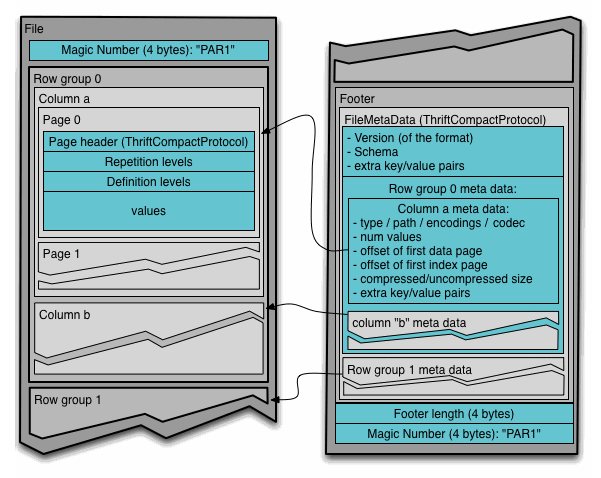
<p>위 그림은 Parquet 파일 하나의 구성을 나타냅니다.
하나의 Parquet 파일은 하나의 테이블 데이터를 담습니다.
파일에는 데이터 영역과 메타데이터 영역이 있습니다.
데이터 영역은 연속된 row group으로 이루어져 있고, 각각의 row group에는 특정 개수 만큼의 레코드(튜플) 데이터가 column chunk로 구분되어 저장되어 있습니다.
하나의 column chunk는 하나의 열(column)에 해당하고, 이것은 여러 개의 페이지로 구성되어 있습니다.
각각의 페이지는 페이지의 정보를 나타내는 페이지 헤더(메타데이터)와 nested 데이터(e.g., JSON, Protobuf, etc.)를 관리하기 위한 repetition levels 및 definition levels (이에 대해서는 이후에 다룹니다), 그리고 실제 데이터를 관리합니다.</p>

<p>메타데이터는 Thrift Protocol [2]로 정의되어 있습니다.
파일의 가장 끝부분에 위치한 파일 메타데이터는 스키마 정보, 각 row group의 정보 (데이터의 위치, 압축 방식 등) 등을 저장합니다.</p>

<p>이런 식으로 데이터를 row group과 column chunk로 나누어 저장하는 방식을 PAX(Partition Attributes Across)라고 합니다.
DuckDB의 storage format도 유사한 방식으로 구성되어 있습니다 [6].</p>

<h3 id="최적화된-쿼리-프로세싱-및-압축">최적화된 쿼리 프로세싱 및 압축</h3>

<p>Parquet는 predicate pushdown 기능을 지원하여 빠른 스캔 성능을 제공하고, 효율적인 압축을 통해 저장 공간을 최적화합니다.
이러한 기능을 위해 Parquet는 <em>zone map</em> (min/max 통계), <em>dictionary encoding</em> (+ <em>run-length encoding</em>과 <em>bit packing</em>), <em>bloom filter</em>, 그리고 다양한 <em>압축 알고리즘</em>을 사용합니다.</p>

<h4 id="zone-map">Zone map</h4>

<p>Parquet는 각각의 row group 내에 있는 column chunk마다 데이터의 min 값과 max 값을 통계 정보로 기록해 두고 있습니다. 이를 <strong>zone map</strong>이라고 합니다. Zone map이 있다면, Parquet 파일에 대해 스캔을 수행할 때, 관련 없는 column chunk에 대한 스캔을 생략할 수 있습니다.</p>

<p>예를 들어 <code class="language-plaintext highlighter-rouge">ORDER BY created_date</code>로 정렬된 주문 데이터가 있다고 가정해보겠습니다. Row Group A는 <code class="language-plaintext highlighter-rouge">created_date</code>의 min=2025-01-01, max=2025-01-31을, Row Group B는 min=2025-02-01, max=2025-02-28을 zone map으로 가지고 있다면, <code class="language-plaintext highlighter-rouge">WHERE created_date &gt;= '2025-02-15'</code>라는 쿼리 실행 시 Row Group A는 스캔하지 않고 건너뛸 수 있습니다.</p>

<p>데이터의 정렬 상태에 따라 zone map의 효과는 매우 클 수 있고, 반대로 매우 작을 수도 있습니다. 만약 데이터가 특정 열을 기준으로 정렬되어 있다면 zone map의 효과는 매우 클 것입니다. 반면 데이터가 정렬되어 있지 않으면서 skewed 되어 있다면, zone map의 효과는 미미할 수 있습니다.</p>

<h4 id="dictionary-encoding">Dictionary encoding</h4>

<p><img src="/assets/images/2025-05-18-apache-parquet-and-opendal/dictionary.png" alt="Dictionary Encoding" width="200" style="display:block; margin-left:auto; margin-right:auto" /></p>

<p style="text-align: center;"><em>Dictionary encoding 예시 [3]</em></p>

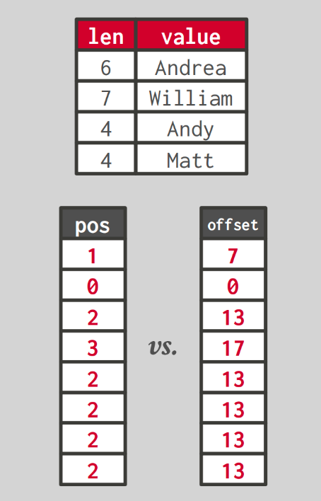
<p><em>Dictionary encoding</em>은 데이터에서 자주 나타나는 값을 dictionary에 저장하고, 데이터는 좀 더 작은 code(예를들어 정수값)로 표현하는 방법입니다.
이 방법은 데이터 압축 측면에서도 좋고, 문자열과 같이 크기가 큰 데이터에 대한 query processing 할 때 유용합니다. 
전체 문자열에 대해 연산을 수행할 필요 없이, code를 이용하여 연산을 수행할 수 있기 때문입니다.
물론 원본 값이 필요할 때에는 그 code에 해당하는 값을 dictionary를 통해 되찾습니다.</p>

<p>대체로 두가지 방식의 code가 사용됩니다. 
하나는 dictionary에 각 데이터 값과 이에 대한 길이를 저장하고, 원본 데이터가 dictionary 내에서 몇번째 index에 저장되어 있는지를 code로 사용하는 방법입니다.
다른 하나는 dictionary에 데이터 값을 연속된 위치에 저장하고, dictionary 내에서 원본 데이터가 몇번째 offset에 저장되어 있는지를 code로 사용하는 방법입니다.
위 그림은 dictionary encoding을 이용하여 문자열을 저장할 때의 이득을 보여주는 예시입니다.
위쪽에는 dictionary가 있고, 왼쪽 아래에는 첫번째 방식의 code, 오른쪽 아래에는 두번째 방식의 code를 이용하여 encoding 한 결과를 보여줍니다.
문자열을 그대로 데이터로 저장한다면 많은 공간을 차지할 수 있지만, 그림과 같이 인코딩하여 관리하면 더 적은 공간으로 처리할 수 있습니다.</p>

<p>Parquet는 <em>run-length encoding</em>과 <em>bitpacking encoding</em>을 dictionary encoding와 함께 사용합니다.
이를 통해 데이터를 추가적으로 압축하여 더욱 효율적인 저장 공간을 확보할 수 있습니다.
Run-length encoding은 반복된 값이 포함된 데이터를 값과 중복된 횟수의 쌍으로 변환합니다.
예를 들어 [1,1,2,2,2,2,3,3]과 같은 데이터가 있을 때 run-length encoding의 결과는 [(1,2),(2,4),(3,2)]가 됩니다.</p>

<p>다른 인코딩 방법 중 하나인 bitpacking encoding은 데이터를 저장할 때 필요한 최소한의 비트만을 사용하여 저장하는 인코딩 방식입니다.
우리가 데이터를 32비트 integer로 표현한다고 할 때, 항상 32비트를 꽉 채워서 사용하는 것은 아닙니다.
만약 우리가 이 데이터의 범위를 알고 있다면(e.g., 페이지 내의 int32 타입 데이터가 0-1000 범위를 가진다면), 우리는 이 정보를 바탕으로 사용하는 비트의 수를 줄일 수 있습니다(e.g., 2¹⁰=1024로 충분히 커버가 가능하므로 10비트+α 로 표현 가능).</p>

<p>Run-length encoding과 bitpacking encoding은 dictionary encoding 없이 데이터에 대해 단독으로 적용될 수도 있습니다.</p>

<p>Parquet는 low cardinality(i.e., distinct한 값의 개수가 적은 경우) 상황일 때 dictionary encoding을 사용합니다.
하나의 열에 같은 값이 많은 경우가 이에 해당하는데, 이 때는 dictionary encoding이 효과적일 것입니다.</p>

<h4 id="bloom-filter">Bloom filter</h4>

<p>위에서 살펴본 zone map이나 dictionary encoding이 효과가 없는 경우가 있을 수 있습니다. 데이터가 large cardinality를 가지면서 매우 skewed 되어 있을 수 있습니다. 그렇다면 이런 경우에는 빠른 스캔을 어떻게 만들어 낼 수 있을까요?</p>

<p>Parquet는 이러한 경우 <em>bloom filter</em> [8]를 사용합니다.
Bloom filter는 특정 원소가 집합에 포함되어 있는지 여부를 확률적으로 판단하는 자료구조입니다.
이것이 “No”를 반환한다면 데이터가 확실히 없는 것이고, “Yes”를 반환한다면 데이터가 있을 수도 있고, 없을 수도 있습니다(False Positive).
Bloom filter는 적은 양의 메모리(데이터 개수 N보다 작은 bits)를 이용하여 “Yes” 혹은 “No” 질의를 빠르게 처리할 수 있습니다.
데이터 저장 시 Parquet는 bloom filter를 만들고, 우리가 데이터를 찾을 때 이 bloom filter를 사용합니다.
만약에 bloom filter가 “Yes”를 반환한다면 해당 column chunk를 스캔해 보는 것이고, “No”를 반환한다면 해당 데이터를 건너뜁니다.</p>

<h4 id="압축">압축</h4>

<p>더 나은 공간 효율성을 위해 Parquet는 다양한 압축 알고리즘을 지원합니다. 대표적으로 <strong>gzip</strong>, <strong>snappy</strong>, <strong>zstd</strong> 등이 있으며, 각각은 압축률과 성능 간의 서로 다른 trade-off를 제공합니다. Gzip은 높은 압축률을 제공하지만 상대적으로 느리고, Snappy는 낮은 압축률을 가지지만 빠른 압축/해제 속도를 제공합니다. Zstd는 두 방식의 중간 지점으로 양호한 압축률과 성능을 모두 제공합니다. 압축은 page 단위로 적용되며, 앞서 언급한 dictionary encoding이나 run-length encoding과 함께 사용되어 더욱 효과적인 압축을 달성할 수 있습니다.</p>

<h3 id="nested-data">Nested Data</h3>

<p>Parquet는 설계 단계에서부터 nested 데이터를 고려하였습니다 [1]. Nested 데이터를 저장 및 관리하기 위해 <strong>Dremel(Google BigQuery)</strong> [9][10]에서 사용한 방법을 채택하였습니다.</p>

<p><img src="/assets/images/2025-05-18-apache-parquet-and-opendal/dremel-nested-concept.png" alt="Dremel Nested Concept" width="500" style="display:block; margin-left:auto; margin-right:auto" /></p>

<p style="text-align: center;"><em>Dremel의 nested 데이터 관리 개념 [9]</em></p>

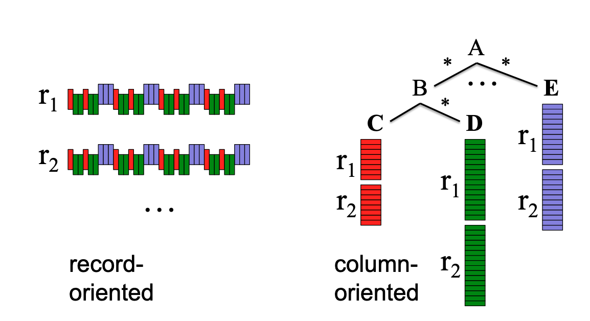
<p>위 그림은 Dremel이 nested 데이터를 관리하는 방법을 개념적으로 나타낸 것입니다.
우측의 트리 구조와 같이 A라는 객체 안에 B, …, E 라는 반복 혹은 생략 가능한 객체가 존재하고, B라는 객체 안에는 C라는 객체와 D라는 반복 혹은 생략 가능한 객체가 존재합니다 (JSON이나 Protobuf와 같은 형태를 생각해 보세요).</p>

<p>이런 객체를 관리하고자 할 때 우리가 데이터를 생긴 그대로 저장한다면, 그림의 좌측과 같이 각각의 nested 객체에 대한 정보가 뒤섞여서 저장되게 됩니다. 반면 Dremel은 열기반 데이터 포맷을 활용하여 우측과 같이 각각의 path에 해당하는 데이터를 연속된 공간에 저장하는 것을 제안했습니다. 후자의 경우 분석 질의를 처리하는 관점에서 더 이득이 있을 것입니다.</p>

<p><img src="/assets/images/2025-05-18-apache-parquet-and-opendal/dremel-nested-method.png" alt="Dremel Nested Method" width="650" style="display:block; margin-left:auto; margin-right:auto" /></p>

<p style="text-align: center;"><em>Dremel의 구체적인 nested 데이터 관리 방법 [10]</em></p>

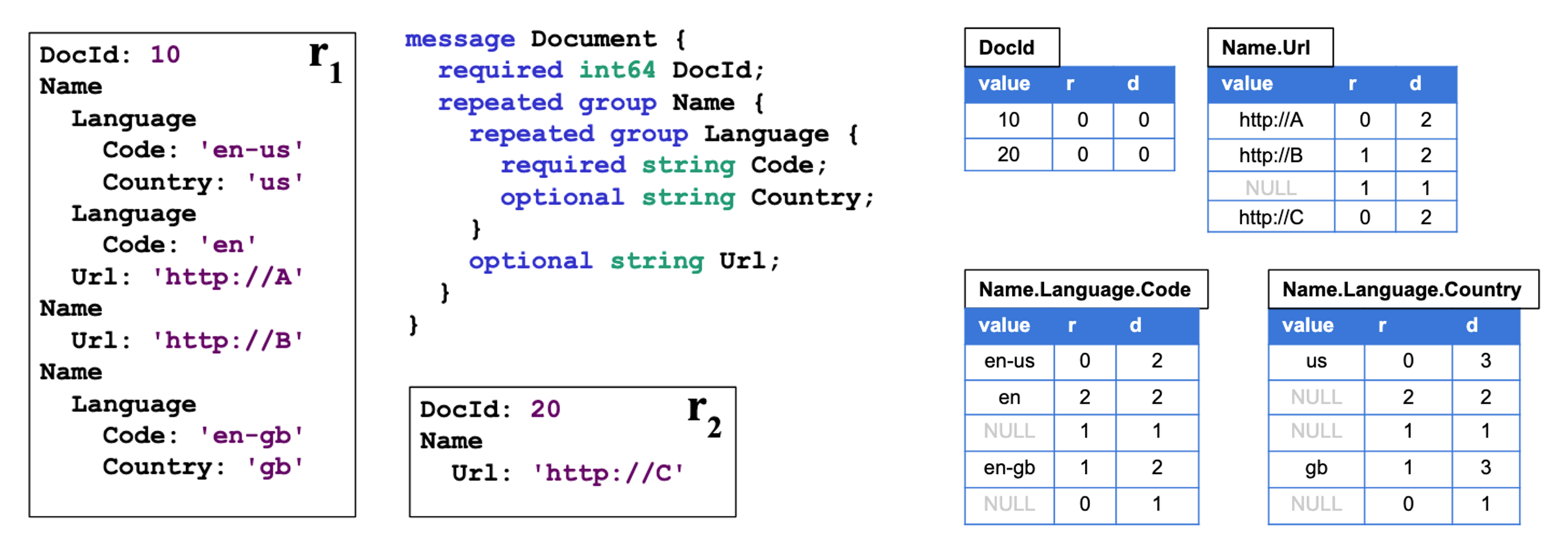
<p>위 그림은 구체적으로 데이터를 어떻게 관리하는지 나타냅니다.
그림의 좌측에는 protobuf의 스키마와 예시 레코드 r₁과 r₂가 있습니다.
Dremel은 스키마의 각각의 path 별로 그림 우측과 같이 분리된 테이블을 생성합니다.</p>

<p>이 테이블에는 해당 필드에 대한 값(value), repetition level 그리고 definition level을 함께 기록해 둡니다.
Repetition level은 현재 튜플과 이전 튜플을 비교했을 때 path 중 어느 depth에서 필드의 반복이 발생하였는지 기록하고 있고, definition level은 현재 튜플이 정의된 path 중 몇개의 optional 필드가 실제로는 정의되었는지 기록하고 있습니다.</p>

<p>Dremel은 nested object를 저장할 때 위와 같은 방식으로 path를 쪼개고 value, repetition level, definition level을 기록합니다. 또한 데이터를 처리해야 하는 시점에는 이 정보들을 활용하여 원본 데이터가 어떻게 생겼는지를 파악하고 데이터를 처리합니다.</p>

<h3 id="더-생각해-볼-주제">더 생각해 볼 주제</h3>

<ul>
  <li>열 기반의 데이터 포맷으로 Apache ORC도 많이 사용되는데, Apache ORC와 Parquet의 차이점은?</li>
  <li>Bloom filter는 range query에도 활용될 수 있을까?</li>
</ul>

<h2 id="apache-opendal">Apache OpenDAL</h2>

<p>OpenDAL은 다양한 스토리지 서비스와 seamless하게 소통할 수 있는 데이터 접근 레이어 입니다.
One layer, all storage를 표방하고 있습니다.</p>

<h3 id="components">Components</h3>

<p>OpenDAL에는 Service, Layer, 그리고 Operator 컴포넌트가 있습니다.</p>

<ul>
  <li>
    <p>Service는 storage backend를 지정하는 컴포넌트입니다.
  AWS S3나 Azure Blob(Azblob)과 같이 bucket service 뿐 아니라 POSIX file system(Fs), PostgreSQL이나 MongoDB 등의 database 접근을 위한 서비스를 제공합니다 [5].</p>
  </li>
  <li>
    <p>Layer는 데이터를 접근할 때 사용할 수 있는 부가적인 기능을 제공합니다.
  데이터에 대한 연산 수행 시 logging을 해주는 <code class="language-plaintext highlighter-rouge">LoggingLayer</code>나 연산 실패 시 자동으로 retry를 수행해주는 <code class="language-plaintext highlighter-rouge">RetryLayer</code>, timeout을 설정해주는 <code class="language-plaintext highlighter-rouge">TimeoutLayer</code> 등을 제공합니다 [7].</p>
  </li>
  <li>
    <p>Operator는 Service에서 지정된 storage에 접근할 수 있도록 합니다.
  Read, write, stat, delete, create_dir, copy 등의 연산을 제공합니다.
  우리는 이를 통해 데이터를 생성하거나 수정, 삭제할 수 있습니다.</p>
  </li>
</ul>

<p>OpenDAL은 현재 특정 범위의 데이터를 읽는 <code class="language-plaintext highlighter-rouge">read_with()</code> 함수는 지원하나, 특정 위치에 데이터를 쓰는 기능(e.g., <code class="language-plaintext highlighter-rouge">pwrite()</code> in POSIX)는 지원하지 않습니다.</p>

<h3 id="databend와의-관계">DataBend와의 관계</h3>

<p>DataBend는 Fuse Engine을 스토리지 엔진으로 사용하며, OpenDAL을 데이터 접근 레이어(data access layer)로 사용합니다.
즉, Fuse Engine은 데이터의 포맷이나 연산을 총괄하는 주체이고, OpenDAL은 그 중에서 데이터를 읽고 쓰는 기능에 집중한다고 할 수 있습니다.</p>

<h3 id="fuse-engine">Fuse Engine</h3>

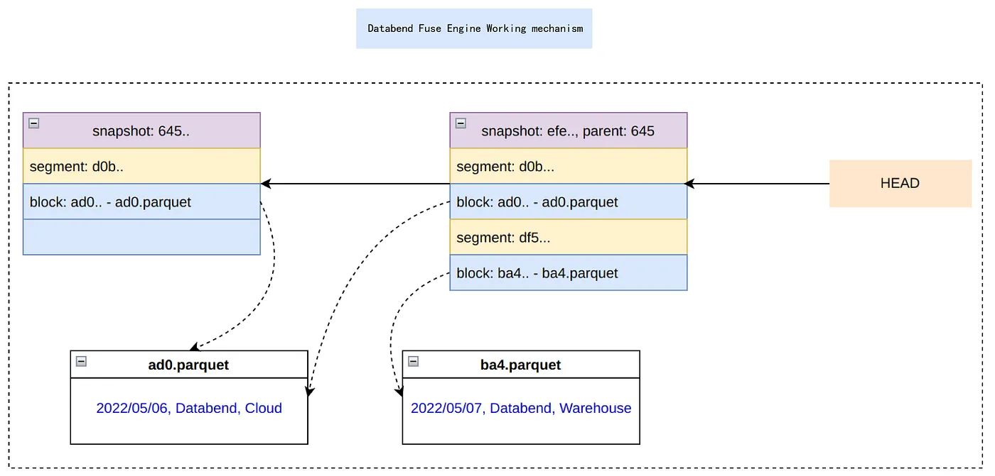
<p><img src="/assets/images/2025-05-18-apache-parquet-and-opendal/fuse.png" alt="Fuse Engine" width="600" style="display:block; margin-left:auto; margin-right:auto" /></p>

<p style="text-align: center;"><em>Fuse Engine의 테이블 관리 메커니즘 [4]</em></p>

<p>위 그림은 Fuse Engine이 하나의 테이블을 관리하는 메커니즘을 표현합니다.
Fuse Engine은 하나의 테이블을 3가지 요소를 통해 관리합니다.</p>

<ul>
  <li>Block: 실제 데이터 조각입니다. Parquet 파일로 구성되어 있습니다.</li>
  <li>Segment: Block들과 이것들의 메타데이터 입니다. 예를 들어 몇 개의 행을 가지고 있는지, 데이터의 사이즈가 어느 정도인지 등을 나타냅니다.</li>
  <li>Snapshot: 특정 시점의 테이블의 상태를 나타내며, Segment들을 포함합니다.</li>
</ul>

<p>테이블이 업데이트(레코드 삽입, 삭제, 수정)될 때마다 새로운 Snapshot이 만들어집니다.
만약 데이터를 포함하는 Block이 변경되어야 한다면 Fuse Engine은 <strong>새로운 Block을 만들어 내고</strong> 이를 포함하는 새로운 Segment와 Snapshot을 만듭니다.
변경되지 않은 Segment나 Block은 테이블이 업데이트 되더라도 새로 만들어지지 않고 기존의 것을 재사용합니다.</p>

<p>Apache Iceberg도 이와 유사한 방식으로 table을 관리합니다.</p>

<h3 id="더-생각해-볼-주제-1">더 생각해 볼 주제</h3>

<ul>
  <li>기존의 RDBMS는 데이터가 업데이트될 때 무슨 일이 일어날까?
(PostgreSQL과 MySQL을 위주로 살펴보기)</li>
  <li>Concurrency control과 performance 측면에서 기존의 RDBMS 방식들과 DataBend의 방식은 어떤 장단점이 있을까?</li>
</ul>

<h2 id="참고문헌">참고문헌</h2>

<p>[1] The Apache Software Foundation. <em>Apache Parquet</em>. 2025. <a href="https://parquet.apache.org/">https://parquet.apache.org/</a></p>

<p>[2] The Apache Software Foundation. <em>Apache Thrift</em>. 2025. <a href="https://thrift.apache.org/">https://thrift.apache.org/</a></p>

<p>[3] Andy Pavlo. <em>Lecture #02: Data Formats &amp; Encoding I</em>. 2024. <a href="https://15721.courses.cs.cmu.edu/spring2024/notes/02-data1.pdf">https://15721.courses.cs.cmu.edu/spring2024/notes/02-data1.pdf</a></p>

<p>[4] DataBend. <em>From Git to Fuse Engine</em>. 2022. <a href="https://medium.com/@databend/from-git-to-fuse-engine-c824b9adea6f">https://medium.com/@databend/from-git-to-fuse-engine-c824b9adea6f</a></p>

<p>[5] OpenDAL. <em>Module services</em>. 2025. <a href="https://docs.rs/opendal/latest/opendal/services/index.html">https://docs.rs/opendal/latest/opendal/services/index.html</a></p>

<p>[6] Mark Raasveldt. <em>Lightweight Compression in DuckDB</em>. 2022. <a href="https://duckdb.org/2022/10/28/lightweight-compression.html">https://duckdb.org/2022/10/28/lightweight-compression.html</a></p>

<p>[7] OpenDAL. <em>Module layers</em>. 2025. <a href="https://docs.rs/opendal/latest/opendal/layers/index.html">https://docs.rs/opendal/latest/opendal/layers/index.html</a></p>

<p>[8] Burton H. Bloom. <em>Space/time trade-offs in hash coding with allowable errors</em>. Communications of the ACM, 13(7):422–426, July 1970.</p>

<p>[9] Sergey Melnik, Andrey Gubarev, Jing Jing Long, Geoffrey Romer, Shiva Shivakumar, Matt Tolton, Theo Vassilakis. <em>Dremel: Interactive Analysis of Web-Scale Datasets</em>. Proc. of the 36th Int’l Conf on Very Large Data Bases, pages 330-339, 2010.</p>

<p>[10] Sergey Melnik, Andrey Gubarev, Jing Jing Long, Geoffrey Romer, Shiva Shivakumar, Matt Tolton, Theo Vassilakis, Hossein Ahmadi, Dan Delorey, Slava Min, and others. <em>Dremel: A decade of interactive SQL analysis at web scale</em>. Proceedings of the VLDB Endowment, 13(12):3461–3472, 2020.</p>]]></content><author><name>Kyoseung Koo</name><email>grammaright@gmail.com</email></author><category term="dbms" /><summary type="html"><![CDATA[이 글은 제가 2025년 5월 18일에 진행한 “Databend 세미나: Topics in Apache Parquet and OpenDAL” 세미나 내용을 기반으로 작성되었습니다.]]></summary></entry><entry><title type="html">Columnar File Format and Storage Access Layer: Technical Analysis of Apache Parquet and OpenDAL</title><link href="https://blog.kyoseung.me/dbms/2025/05/18/apache-parquet-and-opendal.html" rel="alternate" type="text/html" title="Columnar File Format and Storage Access Layer: Technical Analysis of Apache Parquet and OpenDAL" /><published>2025-05-18T10:30:00+00:00</published><updated>2025-05-18T10:30:00+00:00</updated><id>https://blog.kyoseung.me/dbms/2025/05/18/apache-parquet-and-opendal</id><content type="html" xml:base="https://blog.kyoseung.me/dbms/2025/05/18/apache-parquet-and-opendal.html"><![CDATA[<p><em>This post is a translated version of <a href="/dbms/2025/05/18/apache-parquet-and-opendal-ko.html">the blog post</a> originally written in Korean.
This article is based on my seminar “Databend Seminar: Topics in Apache Parquet and OpenDAL” presented on May 18, 2025.</em></p>

<hr />

<h2 id="apache-parquet">Apache Parquet</h2>

<p>Apache Parquet is an open-source column-oriented data file format for efficient data management and retrieval [1]. It was started to provide column-oriented data representation optimized for the Hadoop ecosystem. Parquet’s key characteristics include column-oriented storage, compression, and optimized query processing.</p>

<h3 id="column-oriented-storage">Column-Oriented Storage</h3>

<p><img src="/assets/images/2025-05-18-apache-parquet-and-opendal/parquet-file-layout.png" alt="Parquet File Layout" width="400" style="display:block; margin-left:auto; margin-right:auto" /></p>

<p style="text-align: center;"><em>Internal Structure of a Parquet File [1]</em></p>

<p>The above diagram shows the structure of a single Parquet file.
One Parquet file contains one table’s data.
The file has a data area and metadata areas.
The data area consists of consecutive row groups, and each row group contains data for a specific number of records (tuples) stored as column chunks.
One column chunk corresponds to one column, and it consists of multiple pages.
Each page contains a page header (metadata) that includes page information, repetition and definition levels for managing nested data (e.g., JSON, Protobuf, etc.) (we’ll cover this later), and the actual data.
The metadata located at the end of the file stores schema information and details about each row group like data location and compression method.
The metadata is defined using Thrift Protocol [2].</p>

<p>This method of storing data divided into row groups and column chunks is called PAX (Partition Attributes Across). DuckDB’s storage format is also structured in a similar way [6].</p>

<h3 id="optimized-query-processing-and-compression">Optimized Query Processing and Compression</h3>

<p>Parquet supports predicate pushdown functionality for fast scan performance and optimizes storage space through efficient compression. For these functionalities, Parquet uses <em>zone maps</em> (min/max statistics), <em>dictionary encoding</em> (+ <em>run-length encoding</em> and <em>bit packing</em>), <em>bloom filters</em>, and various <em>compression algorithms</em>.</p>

<h4 id="zone-map">Zone Map</h4>

<p>Parquet records the minimum and maximum values of data as statistical information for each column chunk within each row group.
This is called a <strong>zone map</strong>.
With zone maps, when performing scans on Parquet files, scans of unrelated row groups can be skipped.</p>

<p>For example, suppose we have order data sorted by <code class="language-plaintext highlighter-rouge">ORDER BY created_date</code>. If Row Group A has min=2025-01-01, max=2025-01-31 for <code class="language-plaintext highlighter-rouge">created_date</code>, and Row Group B has min=2025-02-01, max=2025-02-28 in its zone map, then when executing a query like <code class="language-plaintext highlighter-rouge">WHERE created_date &gt;= '2025-02-15'</code>, Row Group A can be skipped without scanning.</p>

<p>Depending on the sorting state of data, the effectiveness of zone maps can be very large or very small. If data is sorted based on a specific column, the zone map’s effectiveness will be very large. Conversely, if data is unsorted and skewed, the zone map’s effectiveness may be minimal.</p>

<h4 id="dictionary-encoding">Dictionary Encoding</h4>

<p><img src="/assets/images/2025-05-18-apache-parquet-and-opendal/dictionary.png" alt="Dictionary Encoding" width="200" style="display:block; margin-left:auto; margin-right:auto" /></p>

<p style="text-align: center;"><em>Dictionary encoding example [3]</em></p>

<p><em>Dictionary encoding</em> is a method that stores frequently appearing values in a dictionary and represents data with smaller codes (e.g., integer values).
This method is good from a data compression perspective and useful for query processing on large-sized data such as strings.
This is because operations can be performed using codes without needing to operate on entire strings.
Of course, when the original value is needed, the corresponding value is retrieved through the dictionary using the code.</p>

<p>Generally, two types of codes are used.
One method stores each data value and its length in the dictionary, and uses which index the original data is stored at in the dictionary as the code.
The other method stores data values in consecutive positions in the dictionary, and uses which offset the original data is stored at within the dictionary as the code.
The above diagram shows an example of the benefits when storing strings using dictionary encoding.
The top shows the dictionary, the bottom left shows the encoding result using the first method’s code, and the bottom right shows the encoding result using the second method’s code.
If strings were stored as data directly, they could take up a lot of space, but by encoding and managing them as shown in the diagram, they can be processed with less space.</p>

<p>Parquet uses <em>run-length encoding</em> and <em>bitpacking encoding</em> together with dictionary encoding.
This allows for additional compression of data to achieve even more efficient storage space.
Run-length encoding converts data containing repeated values into pairs of values and repetition counts.
For example, with data like [1,1,2,2,2,2,3,3], the run-length encoding result would be [(1,2),(2,4),(3,2)].</p>

<p>Another encoding method, bitpacking encoding, uses only the minimum bits needed when storing data.
Even though we represent data as 32-bit integers, we don’t always use all 32 bits.
If we know the range of this data (e.g., if int32 type data within a page have a range of 0-1000), we can reduce the number of bits used based on this information (e.g., since 2¹⁰=1024 provides sufficient coverage, it can be represented with 10 bits+α).</p>

<p>Run-length encoding and bitpacking encoding can be applied to data independently without dictionary encoding.</p>

<p>Parquet uses dictionary encoding in low cardinality situations.
This applies when the same values appear frequently in a column, where dictionary encoding would be effective.</p>

<h4 id="bloom-filter">Bloom Filter</h4>

<p>There may be cases where the zone maps or dictionary encoding explored above are ineffective. Data might have large cardinality while being very skewed. So how can we create fast scans in such cases?</p>

<p>Parquet uses <em>bloom filters</em> [8] for such cases. A bloom filter is a data structure that probabilistically determines whether a specific element is included in a set. If it returns “No,” the data is definitely not there, and if it returns “Yes,” the data may or may not be there (False Positive). Bloom filters can quickly process “Yes” or “No” queries using a small amount of memory (fewer bits than the number of data items N). When storing data, Parquet creates bloom filters, and when we search for data, these bloom filters are used. If the bloom filter returns “Yes,” we scan the corresponding column chunk; if it returns “No,” we skip that data.</p>

<h4 id="compression">Compression</h4>

<p>For better space efficiency, Parquet supports various compression algorithms. These include <strong>gzip</strong>, <strong>snappy</strong>, <strong>zstd</strong>, each providing different trade-offs between compression ratio and performance. Gzip provides high compression ratios but is relatively slow, while Snappy has lower compression ratios but offers fast compression/decompression speeds. Zstd serves as a middle ground, providing both good compression ratios and performance. Compression is applied at the page level, and when combined with the aforementioned dictionary encoding or run-length encoding, it can achieve even more effective compression.</p>

<h3 id="nested-data">Nested Data</h3>

<p>Parquet considered nested data from the design stage [1]. To store and manage nested data, it adopted the method used by <strong>Dremel (Google BigQuery)</strong> [9][10].</p>

<p><img src="/assets/images/2025-05-18-apache-parquet-and-opendal/dremel-nested-concept.png" alt="Dremel Nested Concept" width="500" style="display:block; margin-left:auto; margin-right:auto" /></p>

<p style="text-align: center;"><em>Dremel’s Nested Data Management Concept [9]</em></p>

<p>The above diagram conceptually shows how Dremel manages nested data. Like the tree structure on the right, object A contains repeatable or optional objects B, …, E, and object B contains object C and repeatable or optional object D (think of formats like JSON or Protobuf).</p>

<p>When managing such objects, if we stored data as it appears, information about each nested object would be mixed and stored as shown on the left side of the diagram. In contrast, Dremel proposed using column-oriented data format to store data corresponding to each path in consecutive space as shown on the right. The latter approach would be more advantageous from the perspective of processing analytical queries.</p>

<p><img src="/assets/images/2025-05-18-apache-parquet-and-opendal/dremel-nested-method.png" alt="Dremel Nested Method" width="650" style="display:block; margin-left:auto; margin-right:auto" /></p>

<p style="text-align: center;"><em>Dremel’s Specific Nested Data Management Method [10]</em></p>

<p>The above diagram shows specifically how data is managed. On the left side of the diagram are the protobuf schema and example records r₁ and r₂. Dremel creates separate tables for each path in the schema as shown on the right side of the diagram.</p>

<p>These tables record values for the corresponding fields, repetition levels, and definition levels together.
Repetition levels record at which depth in the path field repetition occurred when comparing the current tuple with the previous tuple, and definition levels record how many optional fields in the paths were actually defined.</p>

<p>When storing nested objects, Dremel splits paths as described above and records values, repetition levels, and definition levels. When data needs to be processed, it uses this information to understand what the original data looked like and processes the data.</p>

<h3 id="further-topics-to-consider">Further Topics to Consider</h3>

<ul>
  <li>Apache ORC is also widely used as a column-oriented data format. What are the differences between Apache ORC and Parquet?</li>
  <li>Can bloom filters also be utilized for range queries?</li>
</ul>

<h2 id="apache-opendal">Apache OpenDAL</h2>

<p>OpenDAL is a data access layer that can communicate seamlessly with various storage services. It advocates “One layer, all storage.”</p>

<h3 id="components">Components</h3>

<p>OpenDAL has Service, Layer, and Operator components.</p>

<ul>
  <li>
    <p>Service is a component that specifies storage backends. It provides access to bucket services like AWS S3 and Azure Blob (Azblob), as well as POSIX file systems (Fs) and database access services like PostgreSQL and MongoDB [5].</p>
  </li>
  <li>
    <p>Layer provides additional functionality that can be used when accessing data. It provides <code class="language-plaintext highlighter-rouge">LoggingLayer</code> for logging during data operations, <code class="language-plaintext highlighter-rouge">RetryLayer</code> for automatic retries on operation failures, <code class="language-plaintext highlighter-rouge">TimeoutLayer</code> for setting timeouts, etc. [7]</p>
  </li>
  <li>
    <p>Operator enables access to storage specified in Service. It provides operations like read, write, stat, delete, create_dir, copy. We can create, modify, or delete data through these operations.</p>
  </li>
</ul>

<p>OpenDAL currently supports the <code class="language-plaintext highlighter-rouge">read_with()</code> function for reading specific ranges of data, but does not support functionality for writing data at specific positions (e.g., <code class="language-plaintext highlighter-rouge">pwrite()</code> in POSIX).</p>

<h3 id="relationship-with-databend">Relationship with DataBend</h3>

<p>DataBend uses Fuse Engine as its storage engine and OpenDAL as its data access layer. In other words, Fuse Engine is the entity that manages data formats and operations, while OpenDAL focuses on reading and writing data functionality.</p>

<h3 id="fuse-engine">Fuse Engine</h3>

<p><img src="/assets/images/2025-05-18-apache-parquet-and-opendal/fuse.png" alt="Fuse Engine" width="600" style="display:block; margin-left:auto; margin-right:auto" /></p>

<p style="text-align: center;"><em>Fuse Engine’s Table Management Mechanism [4]</em></p>

<p>The above diagram represents the mechanism by which Fuse Engine manages a single table. Fuse Engine manages one table through three elements:</p>

<ul>
  <li>Block: Actual data fragments. Composed of Parquet files.</li>
  <li>Segment: Blocks and their metadata. For example, it indicates how many rows they contain, what the data size is, etc.</li>
  <li>Snapshot: Represents the state of a table at a specific point in time and contains Segments.</li>
</ul>

<p>Each time a table is updated (record insertion, deletion, modification), a new Snapshot is created. If a Block containing data needs to be changed, Fuse Engine <strong>creates a new Block</strong> and makes new Segments and Snapshots containing it. Unchanged Segments or Blocks are not recreated when tables are updated but reuse existing ones.</p>

<p>Apache Iceberg also manages tables in a similar way.</p>

<h3 id="further-topics-to-consider-1">Further Topics to Consider</h3>

<ul>
  <li>What happens when data is updated in existing RDBMS? (Focus on PostgreSQL and MySQL)</li>
  <li>What are the advantages and disadvantages of existing RDBMS approaches versus DataBend’s approach in terms of concurrency control and performance?</li>
</ul>

<h2 id="references">References</h2>

<p>[1] The Apache Software Foundation. <em>Apache Parquet</em>. 2025. <a href="https://parquet.apache.org/">https://parquet.apache.org/</a></p>

<p>[2] The Apache Software Foundation. <em>Apache Thrift</em>. 2025. <a href="https://thrift.apache.org/">https://thrift.apache.org/</a></p>

<p>[3] Andy Pavlo. <em>Lecture #02: Data Formats &amp; Encoding I</em>. 2024. <a href="https://15721.courses.cs.cmu.edu/spring2024/notes/02-data1.pdf">https://15721.courses.cs.cmu.edu/spring2024/notes/02-data1.pdf</a></p>

<p>[4] DataBend. <em>From Git to Fuse Engine</em>. 2022. <a href="https://medium.com/@databend/from-git-to-fuse-engine-c824b9adea6f">https://medium.com/@databend/from-git-to-fuse-engine-c824b9adea6f</a></p>

<p>[5] OpenDAL. <em>Module services</em>. 2025. <a href="https://docs.rs/opendal/latest/opendal/services/index.html">https://docs.rs/opendal/latest/opendal/services/index.html</a></p>

<p>[6] Mark Raasveldt. <em>Lightweight Compression in DuckDB</em>. 2022. <a href="https://duckdb.org/2022/10/28/lightweight-compression.html">https://duckdb.org/2022/10/28/lightweight-compression.html</a></p>

<p>[7] OpenDAL. <em>Module layers</em>. 2025. <a href="https://docs.rs/opendal/latest/opendal/layers/index.html">https://docs.rs/opendal/latest/opendal/layers/index.html</a></p>

<p>[8] Burton H. Bloom. <em>Space/time trade-offs in hash coding with allowable errors</em>. Communications of the ACM, 13(7):422–426, July 1970.</p>

<p>[9] Sergey Melnik, Andrey Gubarev, Jing Jing Long, Geoffrey Romer, Shiva Shivakumar, Matt Tolton, Theo Vassilakis. <em>Dremel: Interactive Analysis of Web-Scale Datasets</em>. Proc. of the 36th Int’l Conf on Very Large Data Bases, pages 330-339, 2010.</p>

<p>[10] Sergey Melnik, Andrey Gubarev, Jing Jing Long, Geoffrey Romer, Shiva Shivakumar, Matt Tolton, Theo Vassilakis, Hossein Ahmadi, Dan Delorey, Slava Min, and others. <em>Dremel: A decade of interactive SQL analysis at web scale</em>. Proceedings of the VLDB Endowment, 13(12):3461–3472, 2020.</p>]]></content><author><name>Kyoseung Koo</name><email>grammaright@gmail.com</email></author><category term="dbms" /><summary type="html"><![CDATA[This post is a translated version of the blog post originally written in Korean. This article is based on my seminar “Databend Seminar: Topics in Apache Parquet and OpenDAL” presented on May 18, 2025.]]></summary></entry><entry><title type="html">In-Memory Columnar Storage와 SQL Query Engine: Apache Arrow와 DataFusion의 기술 분석</title><link href="https://blog.kyoseung.me/dbms/2025/04/26/apache-arrow-and-datafusion-ko.html" rel="alternate" type="text/html" title="In-Memory Columnar Storage와 SQL Query Engine: Apache Arrow와 DataFusion의 기술 분석" /><published>2025-04-26T09:00:00+00:00</published><updated>2025-04-26T09:00:00+00:00</updated><id>https://blog.kyoseung.me/dbms/2025/04/26/apache-arrow-and-datafusion-ko</id><content type="html" xml:base="https://blog.kyoseung.me/dbms/2025/04/26/apache-arrow-and-datafusion-ko.html"><![CDATA[<p><em>이 글은 제가 2025년 4월 26일에 진행한 “Databend 세미나: Apache Arrow와 DataFusion의 기술적인 특징과 데이터베이스 시스템과의 관계” 세미나 내용을 기반으로 작성되었습니다.</em></p>

<hr />

<p>이 글에서는 Apache Arrow와 Apache DataFusion의 특징을 살펴보고, 이를 데이터베이스 관리 시스템(DBMS)과 비교하여 논의합니다.</p>

<h2 id="데이터베이스-관리-시스템">데이터베이스 관리 시스템</h2>

<p>먼저 데이터베이스 관리 시스템(Database Management System)이 무엇이고, 여기에 무슨 컴포넌트가 있는지 간략하게 짚고 넘어가겠습니다. 데이터베이스 관리 시스템은 데이터베이스 시스템 또는 간단히 데이터베이스라고도 불립니다. 여기서는 DBMS라고 줄여서 부르도록 하겠습니다.</p>

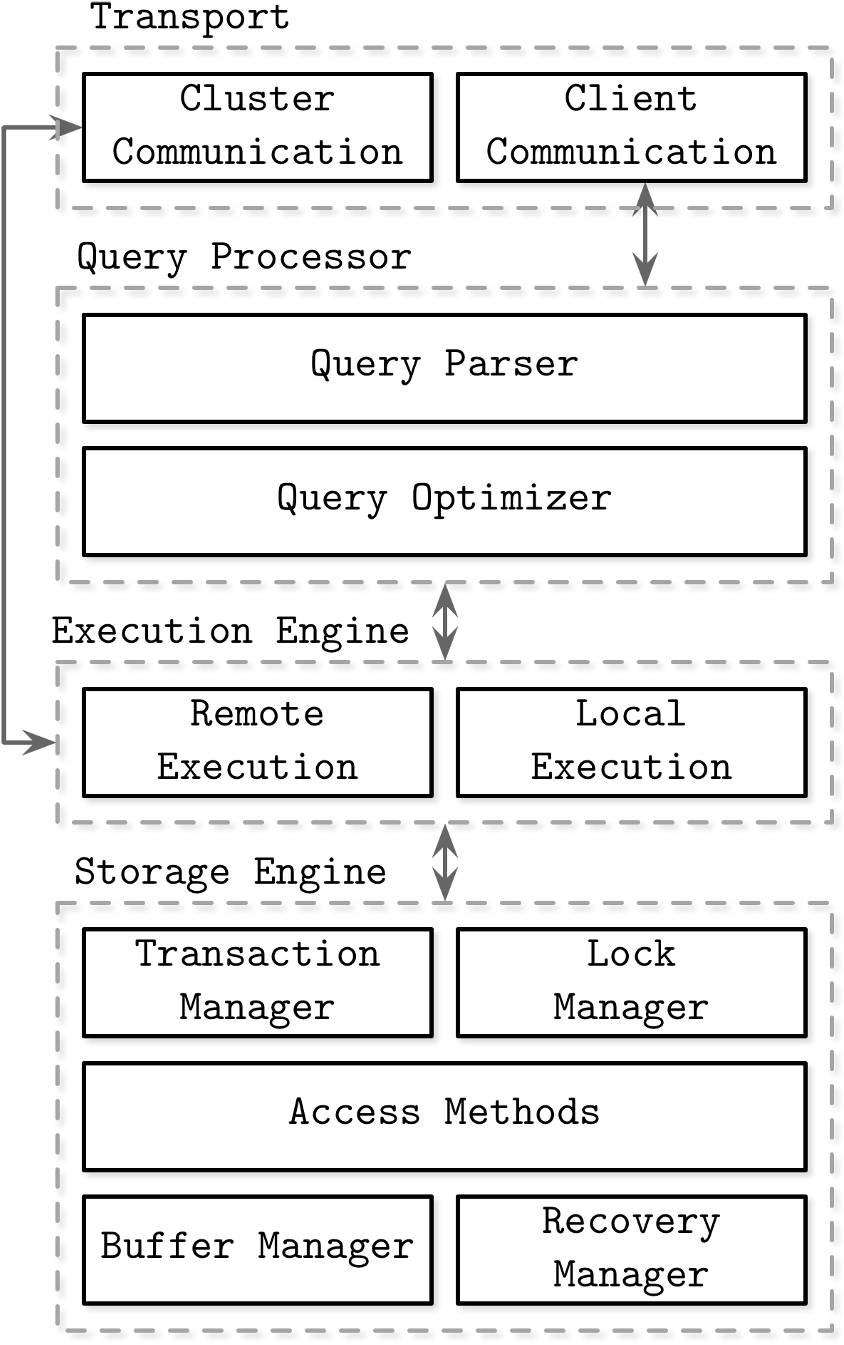
<p><img src="/assets/images/2025-04-26-apache-arrow-and-datafusion/dbms-arch.png" alt="DBMS architecture" width="300" style="display:block; margin-left:auto; margin-right:auto" /></p>

<p style="text-align: center;"><em>DBMS 구성도 개요 (<a href="https://www.oreilly.com/library/view/database-internals/9781492040330/ch01.html">출처</a>)</em></p>

<p>위 그림은 DBMS의 일반적인 아키텍쳐에 대한 이미지입니다.
Transport layer, Query Processor, Execution Engine, Storage Engine을 포함하여 하나의 DBMS라고 혹은 하나의 인스턴스라고 통상 부릅니다.</p>

<p>가장 위의 Transport layer는 클라이언트 프로그램(예: <code class="language-plaintext highlighter-rouge">psql</code>, <code class="language-plaintext highlighter-rouge">mysql</code> 커맨드 프로그램 등)이나 다른 DBMS와의 통신을 담당합니다.
사용자가 클라이언트 프로그램을 통해 쿼리(query 또는 질의)를 입력하면, 해당 쿼리는 DBMS의 Query Processor로 전달됩니다. 관계형 데이터베이스 관리 시스템(Relational Database Management System, 줄여서 RDBMS)의 경우, 통상 Structured Query Language(SQL)을 통해 쿼리를 표현하고, 사용자는 이를 이용하여 쿼리를 요청합니다. 이는 사람이 읽을 수 있는 형태의 언어(human readable language)이기 때문에, Query Parser는 이 SQL을 컴퓨터가 이해하기 위한 형태로 변환합니다.</p>

<p><strong>Query Parser</strong>는 SQL string을 입력받아 컴퓨터가 이해할 수 있는 <strong>logical plan</strong>(논리 계획)을 생성하게 됩니다. 이는 통상 tree(트리)로 나타내며, relational algebra(관계형 대수)를 모방한 내용을 담고 있습니다. Project(<code class="language-plaintext highlighter-rouge">SELECT</code> 절에 해당), Select(<code class="language-plaintext highlighter-rouge">WHERE</code> 절에 해당), Join, Sort 등의 논리적인 연산자가 포함되어 있습니다. 대략 자료구조 시간 때 산술식을 tree로 저장하는 것과 비슷하게 SQL을 tree로 저장하는 역할을 한다고 생각하시면 됩니다.</p>

<p><strong>Query Optimizer</strong>는 이 logical plan을 입력으로 받아 <strong>최적화된 physical plan</strong>(물리 계획; execution plan 혹은 실행 계획이라고도 불림)을 생성합니다. 이 과정에서 이름에 걸맞게 logical plan 혹은 physical plan을 더 좋은 성능을 가지도록 최적화합니다. Physical plan은 logical plan을 어떻게 실행할지에 대한 정보를 포함하고 있습니다. 예를들어 위의 logical plan에는 “Join을 한다”라는 정보를 포함하고 있다면, physical plan에는 “Join을 Hash Join을 통해 처리한다”라는 정보를 포함하고 있습니다.</p>

<p>Execution Engine은 생성된 physical plan을 처리하며, Storage Engine은 디스크 장치에서 데이터를 읽고 쓰면서 Execution Engine을 위한 물리적 데이터 구조를 제공합니다.
<strong>Execution Engine은 Storage Engine이 제공하는 데이터 구조에 따라 쿼리를 처리합니다.</strong> 
예를 들어 column oriented layout을 이용하여 데이터를 관리하는 storage engine을 사용한다면, 내부 데이터 구조 또한 column oriented가 될 것입니다(e.g., <code class="language-plaintext highlighter-rouge">int</code> 타입의 컬럼이라면, <code class="language-plaintext highlighter-rouge">vector&lt;int&gt; columnChunk</code> 와 같은 형태로 데이터를 관리합니다).
그러면 execution engine은 이 데이터 구조를 사용하여 쿼리를 처리하게 됩니다.</p>

<p>이 섹션에서 Query Processor, Execution Engine, Storage Engine의 역할을 간략하게 알아보았습니다. Apache Arrow는 여기에서 Storage Engine의 데이터 관리 형태, Apache DataFusion은 Query Processor와 Execution Engine에 해당한다고 볼 수 있습니다. 자세한 내용을 앞으로 살펴보겠습니다.</p>

<h2 id="apache-arrow">Apache Arrow</h2>

<p>Apache Arrow는 <strong>빠른 데이터 교환</strong> 및 <strong>인메모리 분석</strong>을 위한 <strong>columnar format</strong> 및 <strong>multi-language toolbox</strong> 입니다. 많은 사용자들이 이를 여러 프로세스나 언어간에 연결하는 장치로 사용하거나, 데이터를 빠르게 분석할 수 있는 툴로써 사용합니다.</p>

<p>이 섹션에서는 Apache Arrow의 <strong>1) multi-language를 지원하며 빠르게 데이터를 교환할 수 있고</strong>, <strong>2) columnar in-memory format을 이용하여 데이터를 빠르게 처리할 수 있는</strong> 점에 대해 중점적으로 논의해보도록 하겠습니다.</p>

<h3 id="multi-language-지원-및-빠른-데이터-교환">Multi-language 지원 및 빠른 데이터 교환</h3>

<p>Apache Arrow는 <strong>Zero-copy 데이터 교환</strong>을 통해 데이터를 굉장히 빠르게 옮길 수 있습니다. Zero-copy 데이터 교환이란 데이터를 교환할 때 데이터의 복사를 전혀 하지 않는다는 의미입니다. 우리가 데이터를 특정 프로세스에서 다른 프로세스로 옮기고자 할 때 사용할 수 있는 간편한 방법이 몇가지 있습니다. 데이터를 파일에 쓴 뒤 다른 프로세스에서 읽거나, 통신채널을 열어 데이터를 옮기는 방법이 있습니다. 하지만 이들은 하나의 프로세스가 사용하는 메모리에서 데이터를 disk 혹은 네트워크로 옮기고, 이를 다시 다른 프로세스의 메모리에서 읽어들어야 하는 과정을 수반합니다. 즉, 프로세스의 메모리에서 다른 프로세스의 메모리로 데이터가 copy(복사)되는 것이지요. 데이터의 사이즈가 작을 때에는 이것이 문제되지 않지만, 대규모 데이터 분석과 같이 데이터의 사이즈가 커짐에 따라 데이터 복사에서 발생하는 시간이나 메모리 사용은 궁극적으로 성능 하락으로 이루어질 수 있습니다.</p>

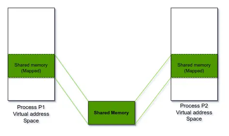
<p><img src="/assets/images/2025-04-26-apache-arrow-and-datafusion/shared-mem.webp" alt="Shared Memory" width="500" style="display:block; margin-left:auto; margin-right:auto" /></p>

<p style="text-align: center;"><em>Shared Memory (<a href="https://medium.com/@rohitkumar_55648/linux-shared-memory-a01c6a8121e">출처</a>)</em></p>

<p>다행히도 이를 해결하는 방법은 우리가 운영체제 시간때 배웠던 <strong>공유메모리(Shared Memory)</strong>를 통해서 해결할 수 있습니다. 위의 그림과 같이 shared memory는 여러 프로세스가 하나의 메모리 공간에 동시에 접근할 수 있도록 합니다. 하나의 프로세스가 메모리 공간에 데이터를 쓰고 다른 프로세스는 그 메모리 공간에 접근하여 데이터를 읽을 수 있게 되는 것이지요. 즉, 데이터 복사 없이 정보를 교환할 수 있게 되는 것입니다.</p>

<p>Apache Arrow는 이러한 공유메모리 기능을 통해 zero-copy 데이터 교환을 실현합니다. Apache Arrow는 공유 메모리를 할당받고 이곳에 자신들의 자료구조나 상태를 설정하며, 이후 모든 데이터는 이 공유 메모리 내에 관리를 하게 됩니다. 추후에 다른 프로세스와 데이터 교환이 필요하다면, 그 프로세스가 공유메모리에 접근할 수 있도록 세팅해주면 됩니다. 물론 서로 다른 프로세스(다른 언어 혹은 다른 시스템)에서 접근하기 위해 공유메모리서 관리되는 자료구조나 상태를 해석할 수 있는 기능이 필요합니다. Apache Arrow는 이것 또한 제공을 하며, 이를 언급하기 위해 <strong>multi-language toolbox</strong>라는 용어를 사용한 것으로 보입니다.</p>

<p>서로 다른 컴퓨터간 데이터 교환하는 경우는 데이터를 다른 컴퓨터로 전송해야 하며, 이는 필연적으로 데이터 복사가 발생하게 됩니다. 이를 위해 Apache Arrow Flight가 사용됩니다.</p>

<p>그럼 Apache Arrow는 어떻게 메모리 상에서 유저의 데이터를 관리할까요? 다음 섹션에서 알아보도록 하겠습니다.</p>

<h3 id="columnar-in-memory-format">Columnar in-memory format</h3>

<p>Apache Arrow는 데이터 교환뿐 아니라 빠른 인메모리 분석 도구로도 유용하게 사용됩니다. 예를들어, Pandas나 Polars와 같은 라이브러리에서 데이터 분석 작업 속도를 향상시키는 데 자주 사용됩니다. 그렇다면 어떻게 Apache Arrow는 이런 성능을 낼 수 있을까요? 여기에는 columnar format이 핵심적인 역할을 하고 있습니다.</p>

<p>Columnar format은 테이블 데이터를 저장하는 방법 중 하나입니다. 전통적인 RDBMS는 테이블 데이터를 row oriented(행 기반) format으로 관리하였습니다. 예를들어 <code class="language-plaintext highlighter-rouge">Student(sid INTEGER, name STRING, age INTEGER)</code>라는 테이블이 있다고 가정해 보겠습니다. Row oriented format의 경우 물리적으로 데이터를 <code class="language-plaintext highlighter-rouge">1,구교승,29$2,배정모,29$3,서정범,30$4,배현모,31</code>과 같은 식으로 각 행에 대한 정보를 연속된 공간에 저장합니다(<code class="language-plaintext highlighter-rouge">,</code>는 열의 구분을, <code class="language-plaintext highlighter-rouge">$</code>은 행의 구분을 위해 사용되었습니다). 반면 column oriented format의 경우 물리적으로 데이터를 <code class="language-plaintext highlighter-rouge">1,2,3,4$구교승,배정모,서정범,배현모$29,29,30,31</code>과 같이 각 열에 대한 정보를 연속된 공간에 저장합니다(<code class="language-plaintext highlighter-rouge">,</code>는 행의 구분을, <code class="language-plaintext highlighter-rouge">$</code>은 열의 구분을 위해 사용되었습니다).</p>

<p>그렇다면 왜 columnar format을 사용할까요? Columnar format은 분석 쿼리를 잘 처리하기 위해 사용됩니다. 분석 쿼리는 대부분 단일 행을 접근하는 것보다는 여러 행을 접근하여 집계를 하는 동작을 수행합니다. <code class="language-plaintext highlighter-rouge">SELECT SUM(age) FROM Student</code>라는 쿼리가 분석 쿼리의 간단한 예시가 될 수 있겠습니다. 이것을 row oriented format으로 처리한다고 가정해 보겠습니다 (이전 단락의 예시와 함께 보세요). DBMS는 물리적으로 저장된 데이터를 읽어들인 뒤에 각 행별로 가장 마지막 column <code class="language-plaintext highlighter-rouge">age</code>를 찾아가 읽어내야 합니다. 그 뒤에 이 값들을 합산하겠지요. 반면 column oriented format으로 처리한다고 생각해 보겠습니다. DBMS는 특정 열를 찾은 뒤에 연속적으로 저장되어 있는 <code class="language-plaintext highlighter-rouge">age</code>값을 한번에 읽어들이기만 하면 됩니다. 이러한 접근 방식의 차이점은 storage의 sequential I/O를 더 적극적으로 활용할 수 있고(연속된 <code class="language-plaintext highlighter-rouge">age</code>값을 읽으면 되기 때문에), CPU의 caching 측면에서도 유리하게 작용합니다. 궁극적으로 성능상 이득이 있는 것이지요.</p>

<p>더 나아가 column format은 요즘 많은 시스템에서 사용하는 vectorized execution에 유리한 조건을 만들어 냅니다. 
Vectorized exectuion은 데이터를 처리할 때 여러 행에 대한 데이터를 한번에 처리하는 것을 의미합니다.
요즘 CPU는 Single Instruction Multiple Data(SIMD) 연산을 지원하는데, 이는 vector processing에 더욱 더 큰 성능 이득을 가져다 줍니다.
Columnar format은 함께 처리해야 하는 데이터가 이미 연속된 공간에 존재하기 때문에(<code class="language-plaintext highlighter-rouge">age</code> 열의 값이 <code class="language-plaintext highlighter-rouge">29,29,30,31</code>과 같이 연속된 공간에 저장), 이러한 SIMD 연산을 위한 최적의 상태에 있습니다.
만약 행 기반의 데이터였다면 loop을 통해 최소 4개 이상의 instruction이 필요했겠지만, SIMD 연산으로는 하나면 충분합니다.
뿐만 아니라 연속된 공간에 데이터가 저장되어 있는 점은 CPU caching 측면에서도 이득을 가져다 줍니다.</p>

<p>Apache Arrow는 이런 columnar format의 장점을 극대화합니다. Apache Arrow 사용자의 데이터를 columnar format으로 메모리 상에서 관리하고, SIMD 연산과 효율적인 구현으로 빠른 데이터 처리 성능을 제공합니다.</p>

<h3 id="더-읽어볼-거리">더 읽어볼 거리</h3>

<ul>
  <li>Apache Arrow의 columnar format은 구체적으로 어떻게 생겼는가? <a href="https://arrow.apache.org/docs/format/Columnar.html#physical-memory-layout">링크</a></li>
  <li>Apache Arrow는 구체적으로 어떻게 IPC를 실현하는가? 어떻게 shared memory를 관리하고 어떤 IPC format으로 데이터 통신을 수행할까? <a href="https://arrow.apache.org/docs/format/Columnar.html#serialization-and-interprocess-communication-ipc">링크</a></li>
  <li>Column Store가 Row Store보다 분석 쿼리에서 더 좋은 성능을 내는 이유는 무엇일까? <a href="https://www.cs.umd.edu/~abadi/papers/abadi-sigmod08.pdf">링크</a></li>
  <li>어떻게 columnar format에서 variable-length type(e.g., VARCHAR)나 nested object(e.g., structure)를 관리할 수 있을까? <a href="https://arrow.apache.org/docs/format/Columnar.html#variable-size-list-layout">variable-length</a>, <a href="https://arrow.apache.org/docs/format/Columnar.html#struct-layout">structured layout</a></li>
</ul>

<h2 id="apache-datafusion">Apache DataFusion</h2>

<p>Apache DataFusion은 <strong>Apache Arrow를 인메모리 포멧</strong>으로 사용하는 <strong>확장성</strong> 있는 <strong>쿼리 엔진</strong>입니다. 즉, columnar format을 기반으로 SQL 질의를 처리하는 엔진이며 이것의 확장성이 좋다는 의미이겠지요. 많은 사용자들은 DataFusion을 자신의 프로세스에 임베딩하여 SQL 혹은 DataFrame engine으로 사용합니다.</p>

<p>DataFusion는 새로운 DBMS를 구축할 때 고품질의 오픈소스 쿼리 엔진을 활용하는 것이 미래의 트렌드가 될 것이라고 제시하고 있습니다 (<a href="https://docs.google.com/presentation/d/1D3GDVas-8y0sA4c8EOgdCvEjVND4s2E7I6zfs67Y4j8/edit#slide=id.g22007bd2b6f_0_343">출처</a>).
전통적으로 각 데이터베이스 시스템이 자체적인 쿼리 엔진을 개발해왔지만 (예를들어 MySQL과 Postgres와 같은 시스템들은 제각각 다른 구성을 가지고 있죠), 이는 구축과 유지보수에 많은 비용이 든다고 분석하고 있습니다.  DataFusion은 새로운 DBMS를 만들 때 처음부터 만들지 말고, DataFusion과 같이 잘 구성된 시스템을 모듈 형식으로 가져가 쓰자고 제안합니다.
그 뒤에 개발하고자 하는 DBMS 특징에 맞게 기능을 추가하거나 코드를 수정하자고 말하죠.</p>

<p>그런 이유인지 DataFusion은 전통적인 DBMS와 매우 유사하게 구성되어 있습니다.
이번 장에서는 어떤 식으로 DataFusion 쿼리 엔진이 구성되어 있는는지 알아보도록 하겠습니다.</p>

<h3 id="query-engine-components">Query Engine Components</h3>

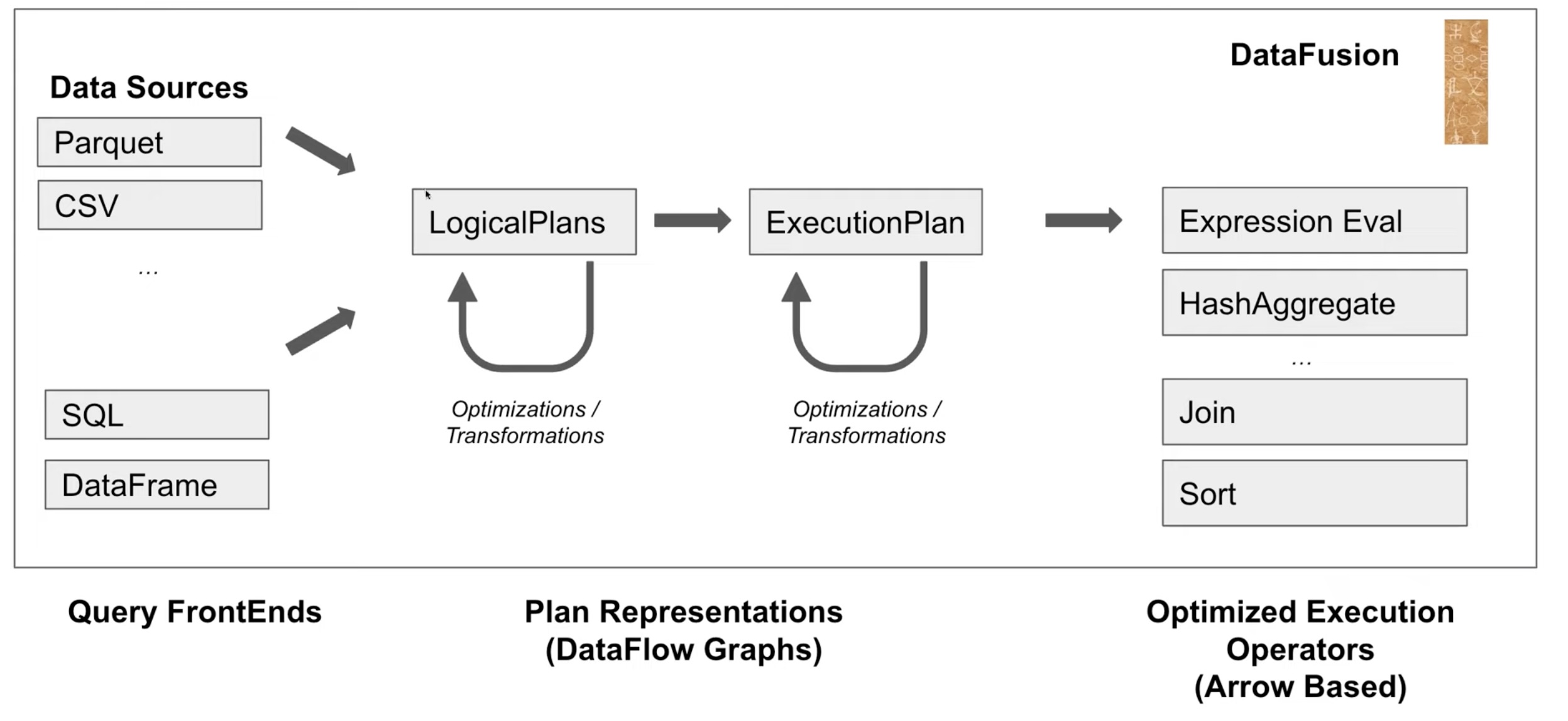
<p><img src="/assets/images/2025-04-26-apache-arrow-and-datafusion/datafusion-arch.jpg" alt="DataFusion architecture" width="600" style="display:block; margin-left:auto; margin-right:auto" /></p>

<p style="text-align: center;"><em>DataFusion 개요 (<a href="https://docs.google.com/presentation/d/1D3GDVas-8y0sA4c8EOgdCvEjVND4s2E7I6zfs67Y4j8/edit#slide=id.p">출처</a>)</em></p>

<p>위 그림은 DataFusion의 구성도를 표현하고 있습니다. 좌측 상단에 있는 것은 Data Sources로, 우리가 맨 처음 살펴본 DBMS 구성에서 Storage Engine이 읽고 쓰는 데이터의 원천입니다. 좌측 하단은 사용자가 SQL과 DataFrame을 이용하여 DataFusion에 쿼리를 할 수 있다는 것을 의미합니다. 그림의 중앙부에는 LogicalPlans과 ExecutionPlan으로 이루어진 Plan Representations가 배치되어 있습니다. 이것은 DBMS 설명에서 논의한 logical plan(논리 계획)과 physical plan(물리 계획)과 동일한 것입니다. 우측에 있는 것은 Optimized Execution Operators로 ExecutionPlan에 포함되어 실행될 수 있는 연산자(operator)를 의미합니다.</p>

<p>그림에서 알 수 있듯이, DataFusion은 DBMS의 쿼리엔진이 하는 것과 동일한 일을 하고 있습니다. FrontEnds로부터 입력된 쿼리를 가공하여 logical plan을 만들고, 이것은 변환(Transformation) 혹은 최적화(Optimization)을 통해 더 나은 logical plan으로 변환됩니다. DataFusion은 생성된 plan을 실제로 어떻게 실행할지를 나타내는 execution plan으로 변환합니다. 이 과정에서 위와 유사하게 변환과 최적화를 수행하게 됩니다. 이후에 Arrow를 기반으로 작성된 연산자를 이용하여 execution plan을 실행합니다.</p>

<h3 id="쿼리-최적화">쿼리 최적화</h3>

<p><img src="/assets/images/2025-04-26-apache-arrow-and-datafusion/datafusion-qo.png" alt="DataFusion Query Optimization" width="600" style="display:block; margin-left:auto; margin-right:auto" /></p>

<p style="text-align: center;"><em>DataFusion Logical Plan Optimization (<a href="https://docs.google.com/presentation/d/1ypylM3-w60kVDW7Q6S99AHzvlBgciTdjsAfqNP85K30/edit#slide=id.p">출처</a>)</em></p>

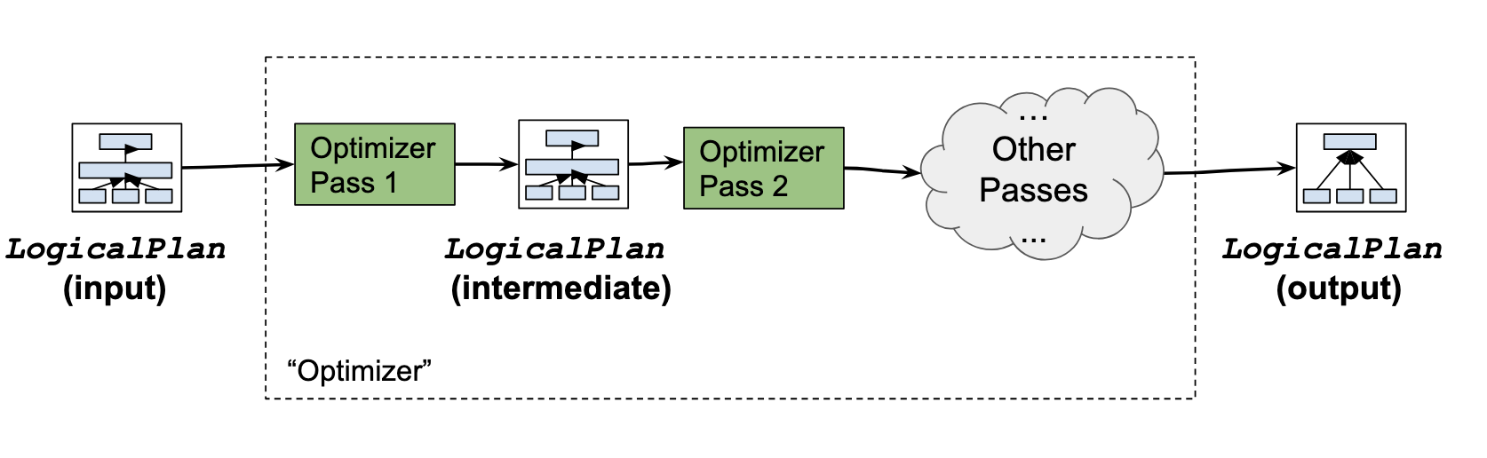
<p>DataFusion의 logical plan 최적화는 위의 그림과 같이 여러 단계로 구성되어 있습니다. Logical plan이 입력으로 주어지면, optimizer pass 1을 통해 조금 더 성능이 개선된 logical plan을 만들고, 그것을 입력으로 optimizer pass 2를 통해 조금 더 성능이 개선된 logical plan을 만들고, 이런 과정을 반복하여 최종 logical plan을 만들어 냅니다. 각각의 optimizer pass는 내장된 rule에 따라 규정이 되어 있으며, 이는 rule의 조건에 맞는지 혹은 예측되는 성능에 따라 결과 logical plan에 반영이 될수도 있고 되지 않을수도 있습니다. 각각의 optimizer pass에는 아래와 같은 일들을 수행합니다.</p>

<ul>
  <li>Pushdown: Projection, Limit, Filter 연산자를 query plan의 시작점 쪽으로 이동</li>
  <li>Simplify-1: 쿼리 실행 중 expression evaluation을 최소화</li>
  <li>Simplify-2: 필요 없는 연산자 제거</li>
  <li>Flatten Subqueries: Nested 쿼리(subquery)를 join으로 대체</li>
  <li>Optimize Joins: Join 연산 최적화</li>
  <li>Optimize DISTINCT: DISTINCT 연산 최적화</li>
</ul>

<p>Execution plan은 위 과정에서 생성된 최종 logical plan으로부터 생성되며, 이 또한 logical plan과 동일하게 여러 optimizer pass를 통해 최적화됩니다. 이 과정에서 적용되는 optimization은 아래와 같습니다.</p>

<ul>
  <li>Enforce Sort/Partitioning: 데이터가 sorting 혹은 partitioning이 필요한지 판단</li>
  <li>Pick Algorithm: sorting/partitioning 여부를 기반으로 join과 sort 연산의 알고리즘을 결정</li>
  <li>Use Statistics: 통계정보를 확인하고 가능한 경우 Scan을 대체</li>
</ul>

<p>DataFusion의 특징 중 하나는 확장성입니다. 이에 걸맞게 쿼리 최적화 기능 또한 사용자가 직접 추가할 수 있습니다. 구체적인 내용은 더 읽어볼 거리에 남겨두도록 하겠습니다.</p>

<h3 id="성능-측면의-특징">성능 측면의 특징</h3>

<p>Apache DataFusion은 빠른 쿼리 실행 성능을 장점으로 내세우고 있습니다. 크게 asynchronous I/O, vectorized processing, partitioning을 통한 multi-core processing이 쿼리 성능에 기여를 합니다.</p>

<p>Asynchronous I/O는 I/O를 비동기식으로 처리하는 것을 의미합니다. I/O의 대상이 되는 disk나 network의 경우, CPU에 비해 엄청나게 느리게 동작합니다. 따라서 CPU가 I/O를 요청하게 되면 요청이 처리될 때 까지 (즉, HDD에서 데이터를 읽거나, 네트워크를 통해 데이터를 성공적으로 전송할 때 까지) CPU는 할 일이 없게 됩니다. 이 때 CPU가 다른 일을 하지 않고 기다리는 것을 Synchronous I/O라고 하고, 그 사이에 다른 일을 하는 것을 Asynchronous I/O라고 합니다. DataFusion은 Async I/O 방식을 채택하여 사용하고 있습니다.</p>

<p>Vectorized processing은 이전 장에서 설명한 것처럼 columnar format과 궁합이 잘 맞습니다. 
DataFusion은 columnar 방식인 Arrow를 기반으로 하여 좋은 성능을 냅니다.</p>

<p><img src="/assets/images/2025-04-26-apache-arrow-and-datafusion/datafusion-partition.png" alt="DataFusion Data Partitioning" width="700" style="display:block; margin-left:auto; margin-right:auto" /></p>

<p style="text-align: center;"><em>DataFusion Data Partitioning (<a href="https://docs.google.com/presentation/d/1cA2WQJ2qg6tx6y4Wf8FH2WVSm9JQ5UgmBWATHdik0hg/edit#slide=id.g209d99697c0_0_11">출처</a>)</em></p>

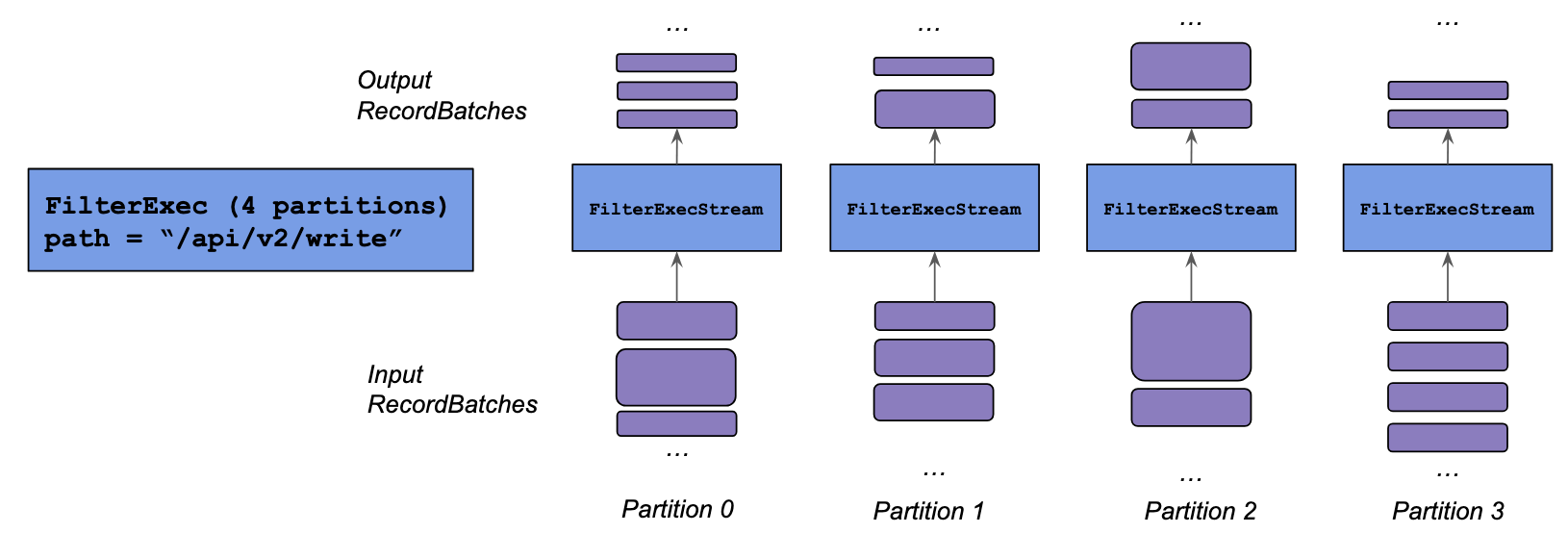
<p>DBMS 맥락에서 partitioning은 데이터를 특정한 기준에 맞게 물리적으로 그룹화 하는 것을 의미합니다. DataFusion은 위의 그림과 같이 데이터를 partition으로 쪼갠 뒤에, data-parallel 한 방식을 이용하여 쿼리를 수행합니다.</p>

<p>여기까지 DataFusion에 대해서 알아보았습니다.
독자들에게 유용할 수 있을 링크를 더 읽어볼 거리에 추가하였으니 기회가 된다면 살펴보시기 바랍니다.</p>

<h3 id="더-읽어볼-거리-1">더 읽어볼 거리</h3>

<ul>
  <li>DataFusion은 어떻게 각각의 연산자를 호출하고 데이터를 생성할까? 구체적으로 어떤 query execution model을 사용할까? <a href="https://docs.rs/datafusion/latest/datafusion/#execution">Volcano-style query execution model</a></li>
  <li>DataFusion은 구체적으로 어떻게 쿼리를 최적화할까? <a href="https://datafusion.apache.org/library-user-guide/query-optimizer.html">doc</a>, <a href="https://github.com/apache/datafusion/tree/main/datafusion/optimizer">code</a></li>
  <li>어떻게 사용자 정의 쿼리 최적화 룰을 추가할 수 있을까? <a href="https://datafusion.apache.org/library-user-guide/query-optimizer.html#writing-optimization-rules">링크</a></li>
  <li>어떻게 사용자 정의 함수 및 집계를 추가할 수 있을까? <a href="https://datafusion.apache.org/python/user-guide/common-operations/udf-and-udfa.html">링크</a></li>
</ul>

<h2 id="마치는-말">마치는 말</h2>

<p>DBMS를 중점적으로 연구/개발하는 사람들은 최근 DataFusion과 Arrow를 포함하는 Flight DataFusion Arrow Parquet stack(줄여서 FDAP stack)에 관심이 많은 것 같습니다. 특히 이 stack을 이용해서 DBMS를 새로 만드는 것에 말입니다. 대표적인 예시로 InfluxDB의 경우 버전 2까지는 자신들이 개발하던 아키텍처를 사용했지만, 버전 3는 FDAP stack으로 새로운 시스템을 개발했다고 합니다 (<a href="https://youtu.be/AGS4GNGDK_4?si=61Kom1xSWZAFlmTa">출처</a>).</p>

<p>지금까지 FDAP stack에서 Apache Arrow와 DataFusion의 기술적인 특징에 대하여 논의하였습니다.
이는 DBMS의 Query Engine(Query Processor 및 Execution Engine)과 Storage Engine의 일부를 커버하고 있습니다.
<a href="/dbms/2025/05/18/apache-parquet-and-opendal-ko.html">다음 글</a>에서는 더 아래단의 Storage Engine과 밀접한 Parquet에 대해서 살펴보도록 하겠습니다. 또한 여러 data format을 통합된 레이어로 읽을 수 있는 OpenDAL에 대해서도 살펴보도록 하겠습니다.</p>]]></content><author><name>Kyoseung Koo</name><email>grammaright@gmail.com</email></author><category term="dbms" /><summary type="html"><![CDATA[이 글은 제가 2025년 4월 26일에 진행한 “Databend 세미나: Apache Arrow와 DataFusion의 기술적인 특징과 데이터베이스 시스템과의 관계” 세미나 내용을 기반으로 작성되었습니다.]]></summary></entry><entry><title type="html">In-Memory Columnar Storage and SQL Query Engine: Technical Analysis of Apache Arrow and DataFusion</title><link href="https://blog.kyoseung.me/dbms/2025/04/26/apache-arrow-and-datafusion.html" rel="alternate" type="text/html" title="In-Memory Columnar Storage and SQL Query Engine: Technical Analysis of Apache Arrow and DataFusion" /><published>2025-04-26T09:00:00+00:00</published><updated>2025-04-26T09:00:00+00:00</updated><id>https://blog.kyoseung.me/dbms/2025/04/26/apache-arrow-and-datafusion</id><content type="html" xml:base="https://blog.kyoseung.me/dbms/2025/04/26/apache-arrow-and-datafusion.html"><![CDATA[<p><em>This post is a translated version of <a href="/dbms/2025/04/26/apache-arrow-and-datafusion-ko.html">the blog post</a> originally written in Korean.
This article is based on my seminar “Databend Seminar: Technical Features of Apache Arrow and DataFusion and their Relationship with Database Systems” presented on April 26, 2025.</em></p>

<hr />

<p>This article examines the characteristics of Apache Arrow and Apache DataFusion, discussing them in comparison with Database Management Systems (DBMS).</p>

<h2 id="database-management-systems">Database Management Systems</h2>

<p>First, let’s briefly overview what a Database Management System is and what components it contains. A Database Management System is also called a database system or simply a database. Here, I’ll use the abbreviation DBMS.</p>

<p><img src="/assets/images/2025-04-26-apache-arrow-and-datafusion/dbms-arch.png" alt="DBMS architecture" width="300" style="display:block; margin-left:auto; margin-right:auto" /></p>

<p style="text-align: center;"><em>DBMS Architecture Overview (<a href="https://www.oreilly.com/library/view/database-internals/9781492040330/ch01.html">source</a>)</em></p>

<p>The above diagram shows a typical DBMS architecture.
These components are collectively referred to as a single DBMS or instance.</p>

<p>The topmost Transport layer handles communication with client programs (e.g., <code class="language-plaintext highlighter-rouge">psql</code>, <code class="language-plaintext highlighter-rouge">mysql</code> command programs) and other DBMS instances.
When a user inputs a query through a client program, that query is passed to the DBMS’s Query Processor. In the case of Relational Database Management Systems (RDBMS), queries are typically expressed using Structured Query Language (SQL), which users use to make query requests. Since this is a human readable language, the Query Parser converts this SQL into a form that computers can understand.</p>

<p>The <strong>Query Parser</strong> takes an SQL string as input and generates a <strong>logical plan</strong> that computers can understand. This is typically represented as a tree containing relational algebra operations. It includes logical operators such as Project (corresponding to <code class="language-plaintext highlighter-rouge">SELECT</code> clauses), Select (corresponding to <code class="language-plaintext highlighter-rouge">WHERE</code> clauses), Join, and Sort. Think of it roughly like storing arithmetic expressions as trees in data structures class, but for SQL.</p>

<p>The <strong>Query Optimizer</strong> takes this logical plan as input and generates an <strong>optimized physical plan</strong> (also called an execution plan). In this process, it optimizes the logical plan or physical plan to achieve better performance. The physical plan contains information about how to execute the logical plan. For example, while the logical plan contains information like “perform a Join,” the physical plan contains information like “process the Join using Hash Join.”</p>

<p>The Execution Engine processes the generated physical plan. 
Meanwhile, the Storage Engine reads and writes data to and from disk devices, providing the Execution Engine with the necessary physical data structure.
<strong>The Execution Engine then processes queries based on this structure.</strong> 
For example, if a storage engine uses a column-oriented layout to manage data, its internal data structures will also be column-oriented (e.g., for an <code class="language-plaintext highlighter-rouge">int</code> column, the internal data structure looks like <code class="language-plaintext highlighter-rouge">vector&lt;int&gt; columnChunk</code>). 
The Execution Engine can then use these data structures to efficiently process a query.</p>

<p>In this section, we briefly explored the roles of Query Processor, Execution Engine, and Storage Engine. Apache Arrow corresponds to the data management format of the Storage Engine, while Apache DataFusion corresponds to the Query Processor and Execution Engine. Let’s examine the details ahead.</p>

<h2 id="apache-arrow">Apache Arrow</h2>

<p>Apache Arrow is a <strong>columnar format</strong> and <strong>multi-language toolbox</strong> for <strong>fast data exchange</strong> and <strong>in-memory analytics</strong>. Many users use it as a bridge between different processes or languages, or as a tool for fast data analysis.</p>

<p>This section will focus on Apache Arrow’s ability to <strong>1) support multi-language and fast data exchange</strong>, and <strong>2) process data quickly using columnar in-memory format</strong>.</p>

<h3 id="multi-language-support-and-fast-data-exchange">Multi-language Support and Fast Data Exchange</h3>

<p>Apache Arrow can move data extremely fast through <strong>Zero-copy data exchange</strong>. Zero-copy data exchange means no data copying occurs during data exchange. When we want to move data from one process to another, there are several convenient methods available. We can write data to a file and read it from another process, or open a communication channel to transfer data. However, these methods involve moving data from one process’s memory to disk or network, then reading it back into another process’s memory. In other words, data is copied from one process’s memory to another process’s memory. While this isn’t problematic for small data sizes, as data sizes grow in large-scale data analysis, the time spent on data copying and memory usage can ultimately lead to performance degradation.</p>

<p><img src="/assets/images/2025-04-26-apache-arrow-and-datafusion/shared-mem.webp" alt="Shared Memory" width="500" style="display:block; margin-left:auto; margin-right:auto" /></p>

<p style="text-align: center;"><em>Shared Memory (<a href="https://medium.com/@rohitkumar_55648/linux-shared-memory-a01c6a8121e">source</a>)</em></p>

<p>Fortunately, this can be solved using <strong>Shared Memory</strong>, which we learned about in operating systems class. As shown in the diagram above, shared memory allows multiple processes to access a single memory space simultaneously. One process can write data to the memory space while another process can access that memory space to read the data. This enables information exchange without data copying.</p>

<p>Apache Arrow realizes zero-copy data exchange through this shared memory functionality. Apache Arrow allocates shared memory and sets up its data structures and states there, with all subsequent data managed within this shared memory. Later, when data exchange with other processes is needed, we simply need to set up access to the shared memory for those processes. Of course, for access from different processes (different languages or systems), functionality to interpret the data structures and states managed in shared memory is needed. Apache Arrow provides this as well, which seems to be why they use the term <strong>multi-language toolbox</strong>.</p>

<p>For data exchange between different computers, data must be transmitted to other computers, which inevitably involves data copying. Apache Arrow Flight is used for this purpose.</p>

<p>So how does Apache Arrow manage user data in memory? Let’s explore this in the next section.</p>

<h3 id="columnar-in-memory-format">Columnar In-Memory Format</h3>

<p>Apache Arrow is useful not only for data exchange but also as a fast in-memory analytics tool. For example, it’s frequently used to improve data analysis task performance in libraries like Pandas and Polars. So how can Apache Arrow achieve such performance? The columnar format plays a key role here.</p>

<p>Columnar format is one method of storing table data. Traditional RDBMS managed table data in row-oriented format. For example, consider a table <code class="language-plaintext highlighter-rouge">Student(sid INTEGER, name STRING, age INTEGER)</code>. In row-oriented format, data is physically stored like <code class="language-plaintext highlighter-rouge">1,John Smith,29$2,Jane Doe,29$3,Bob Johnson,30$4,Alice Wilson,31</code>, where information for each row is stored in consecutive space (<code class="language-plaintext highlighter-rouge">,</code> separates columns, <code class="language-plaintext highlighter-rouge">$</code> separates rows). In contrast, column-oriented format physically stores data like <code class="language-plaintext highlighter-rouge">1,2,3,4$John Smith,Jane Doe,Bob Johnson,Alice Wilson$29,29,30,31</code>, where information for each column is stored in consecutive space (<code class="language-plaintext highlighter-rouge">,</code> separates rows, <code class="language-plaintext highlighter-rouge">$</code> separates columns).</p>

<p>So why use columnar format? Columnar format is used to handle analytical queries well. Analytical queries typically perform aggregations by accessing multiple rows rather than accessing single rows. <code class="language-plaintext highlighter-rouge">SELECT SUM(age) FROM Student</code> would be a simple example of an analytical query. Let’s assume this is processed with row-oriented format (refer to the previous paragraph’s example). The DBMS must read the physically stored data, then find and read the last column <code class="language-plaintext highlighter-rouge">age</code> for each row, then sum these values. Now consider processing with column-oriented format. The DBMS simply needs to find a specific column and read all consecutive <code class="language-plaintext highlighter-rouge">age</code> values at once. This difference in approach allows more aggressive use of storage’s sequential I/O and is advantageous from a CPU caching perspective. Ultimately, there are performance benefits.</p>

<p>Furthermore, column format creates favorable conditions for vectorized execution that many modern systems use.
Vectorized execution means processing data for multiple rows at once.
Modern CPUs support Single Instruction Multiple Data (SIMD) operations, which provide even greater performance benefits for vector processing.
Since columnar format already has data that needs to be processed together in consecutive space (<code class="language-plaintext highlighter-rouge">age</code> column values stored consecutively like <code class="language-plaintext highlighter-rouge">29,29,30,31</code>), it’s in an optimal state for such SIMD operations.
If it were row-based data, at least 4 or more instructions would be needed through loops, but with SIMD operations, one is sufficient.
Moreover, having data stored in consecutive space also provides benefits from a CPU caching perspective.</p>

<p>Apache Arrow maximizes these advantages of columnar format. Apache Arrow manages data in columnar format in memory and provides fast data processing performance through SIMD operations and efficient implementation.</p>

<h3 id="further-reading">Further Reading</h3>

<ul>
  <li>What does Apache Arrow’s columnar format specifically look like? <a href="https://arrow.apache.org/docs/format/Columnar.html#physical-memory-layout">Link</a></li>
  <li>How does Apache Arrow specifically implement IPC? How does it manage shared memory and what IPC format does it use for data communication? <a href="https://arrow.apache.org/docs/format/Columnar.html#serialization-and-interprocess-communication-ipc">Link</a></li>
  <li>Why do column stores perform better than row stores for analytical queries? <a href="https://www.cs.umd.edu/~abadi/papers/abadi-sigmod08.pdf">Link</a></li>
  <li>How can variable-length types (e.g., VARCHAR) or nested objects (e.g., structures) be managed in columnar format? <a href="https://arrow.apache.org/docs/format/Columnar.html#variable-size-list-layout">variable-length</a>, <a href="https://arrow.apache.org/docs/format/Columnar.html#struct-layout">structured layout</a></li>
</ul>

<h2 id="apache-datafusion">Apache DataFusion</h2>

<p>Apache DataFusion is an <strong>extensible</strong> <strong>query engine</strong> that uses <strong>Apache Arrow as its in-memory format</strong>.
In other words, it’s an engine that processes SQL queries based on columnar format, and it’s highly extensible.
Many users embed DataFusion into their processes to use it as a SQL or DataFrame engine.</p>

<p>DataFusion proposes that utilizing high-quality open-source query engines will become a future trend when building new DBMS (<a href="https://docs.google.com/presentation/d/1D3GDVas-8y0sA4c8EOgdCvEjVND4s2E7I6zfs67Y4j8/edit#slide=id.g22007bd2b6f_0_343">source</a>).
Traditionally, each database system has developed its own query engine (for example, systems like MySQL and PostgreSQL each have their own distinct architectures), but such approaches require significant costs for development and maintenance. DataFusion proposes that when creating new DBMS, instead of starting from scratch, you should take well-designed systems like DataFusion in modular form.
Then add features or modify code to match the characteristics of the DBMS you want to develop.</p>

<p>Perhaps for this reason, DataFusion is structured very similarly to traditional DBMS.
In this chapter, let’s explore how the DataFusion query engine is structured.</p>

<h3 id="query-engine-components">Query Engine Components</h3>

<p><img src="/assets/images/2025-04-26-apache-arrow-and-datafusion/datafusion-arch.jpg" alt="DataFusion architecture" width="600" style="display:block; margin-left:auto; margin-right:auto" /></p>

<p style="text-align: center;"><em>DataFusion Overview (<a href="https://docs.google.com/presentation/d/1D3GDVas-8y0sA4c8EOgdCvEjVND4s2E7I6zfs67Y4j8/edit#slide=id.p">source</a>)</em></p>

<p>The above diagram represents DataFusion’s architecture.
The upper left shows Data Sources, which are the ones that the Storage Engine reads and writes.
The lower left shows that users can query DataFusion using SQL and DataFrames.
In the center of the diagram, Plan Representations consisting of LogicalPlans and ExecutionPlan are placed.
These are the same as the logical plans and physical plans discussed in the DBMS discussion.
On the right are Optimized Execution Operators, which refer to the operators that can be executed contained in ExecutionPlan.</p>

<p>As you can see from the diagram, DataFusion does the same work as a DBMS query engine. It processes queries input from FrontEnds to create logical plans, which are converted to better logical plans through transformation or optimization. DataFusion converts the generated plan to an execution plan that represents how to actually execute it. In this process, it performs similar transformation and optimization. Then it executes the execution plan using operators written based on Arrow.</p>

<h3 id="query-optimization">Query Optimization</h3>

<p><img src="/assets/images/2025-04-26-apache-arrow-and-datafusion/datafusion-qo.png" alt="DataFusion Query Optimization" width="600" style="display:block; margin-left:auto; margin-right:auto" /></p>

<p style="text-align: center;"><em>DataFusion Logical Plan Optimization (<a href="https://docs.google.com/presentation/d/1ypylM3-w60kVDW7Q6S99AHzvlBgciTdjsAfqNP85K30/edit#slide=id.p">source</a>)</em></p>

<p>DataFusion’s logical plan optimization consists of multiple stages as shown in the diagram above. When a logical plan is given as input, optimizer pass 1 creates a logical plan with slightly improved performance, which serves as input to optimizer pass 2 to create another logical plan with slightly improved performance, and this process repeats to create the final logical plan. 
Each optimizer pass is governed by built-in rules, which may or may not be reflected in the resulting logical plan depending on whether rule conditions are met or predicted performance of the optimized plan is better.
Each optimizer pass performs the following tasks:</p>

<ul>
  <li>Pushdown: Moving Projection, Limit, Filter operators toward the beginning of the query plan</li>
  <li>Simplify-1: Minimizing expression evaluation during query execution</li>
  <li>Simplify-2: Removing unnecessary operators</li>
  <li>Flatten Subqueries: Replacing nested queries (subqueries) with joins</li>
  <li>Optimize Joins: Join operation optimization</li>
  <li>Optimize DISTINCT: DISTINCT operation optimization</li>
</ul>

<p>The execution plan is generated from the final logical plan created through the above process, and this is also optimized through multiple optimizer passes like the logical plan. The optimizations applied in this process include:</p>

<ul>
  <li>Enforce Sort/Partitioning: Determining if data needs sorting or partitioning</li>
  <li>Pick Algorithm: Deciding algorithms for join and sort operations based on sorting/partitioning status</li>
  <li>Use Statistics: Checking statistical information and replacing Scan when possible</li>
</ul>

<p>One of DataFusion’s characteristics is extensibility. Accordingly, users can directly add query optimization functionality. Specific details will be left in the further reading section.</p>

<h3 id="performance-aspects">Performance Aspects</h3>

<p>Apache DataFusion touts fast query execution performance as an advantage. Primarily, asynchronous I/O, vectorized processing, and multi-core processing through partitioning contribute to query performance.</p>

<p>Asynchronous I/O means processing I/O asynchronously. I/O targets like disks or networks operate much slower than CPUs. Therefore, when a CPU requests I/O, the CPU has nothing to do until the request is processed (i.e., until data is read from HDD or successfully transmitted over network). When the CPU waits without doing other work during this time, it’s called Synchronous I/O, and when it does other work meanwhile, it’s called Asynchronous I/O. DataFusion adopts the Async I/O approach.</p>

<p>Vectorized processing works well with columnar format as explained in the previous chapter.
DataFusion achieves good performance by utilizing Apache Arrow’s columnar format.</p>

<p><img src="/assets/images/2025-04-26-apache-arrow-and-datafusion/datafusion-partition.png" alt="DataFusion Data Partitioning" width="700" style="display:block; margin-left:auto; margin-right:auto" /></p>

<p style="text-align: center;"><em>DataFusion Data Partitioning (<a href="https://docs.google.com/presentation/d/1cA2WQJ2qg6tx6y4Wf8FH2WVSm9JQ5UgmBWATHdik0hg/edit#slide=id.g209d99697c0_0_11">source</a>)</em></p>

<p>In the DBMS context, partitioning means physically grouping data according to specific criteria. DataFusion splits data into partitions, then performs queries using a data-parallel approach (as shown in the diagram above).</p>

<p>This concludes our exploration of DataFusion.
I have added links that may be useful to readers in the further reading section, so please take a look.</p>

<h3 id="further-reading-1">Further Reading</h3>

<ul>
  <li>How does DataFusion call each operator and generate data? What specific query execution model does it use? <a href="https://docs.rs/datafusion/latest/datafusion/#execution">Volcano-style query execution model</a></li>
  <li>How does DataFusion specifically optimize queries? <a href="https://datafusion.apache.org/library-user-guide/query-optimizer.html">doc</a>, <a href="https://github.com/apache/datafusion/tree/main/datafusion/optimizer">code</a></li>
  <li>How can you add custom query optimization rules? <a href="https://datafusion.apache.org/library-user-guide/query-optimizer.html#writing-optimization-rules">Link</a></li>
  <li>How can you add custom functions and aggregations? <a href="https://datafusion.apache.org/python/user-guide/common-operations/udf-and-udfa.html">Link</a></li>
</ul>

<h2 id="conclusion">Conclusion</h2>

<p>People who research/develop DBMS seem to be very interested in the Flight DataFusion Arrow Parquet stack (abbreviated as FDAP stack) recently, including DataFusion and Arrow. Particularly in using this stack to create new DBMS. A representative example is InfluxDB, which used its own developed architecture up to version 2, but developed a new system with the FDAP stack for version 3 (<a href="https://youtu.be/AGS4GNGDK_4?si=61Kom1xSWZAFlmTa">source</a>).</p>

<p>So far, we’ve discussed the technical characteristics of Apache Arrow and DataFusion in the FDAP stack. These cover the Query Engine (Query Processor and Execution Engine) and parts of the Storage Engine in DBMS. In the <a href="/dbms/2025/05/18/apache-parquet-and-opendal.html">next article</a>, we’ll examine Parquet, which is closely related to the lower-level Storage Engine. We’ll also look at OpenDAL, a layer that can read various data formats through a unified interface.</p>]]></content><author><name>Kyoseung Koo</name><email>grammaright@gmail.com</email></author><category term="dbms" /><summary type="html"><![CDATA[This post is a translated version of the blog post originally written in Korean. This article is based on my seminar “Databend Seminar: Technical Features of Apache Arrow and DataFusion and their Relationship with Database Systems” presented on April 26, 2025.]]></summary></entry><entry><title type="html">Vectorization and Options for DuckDB Table Function</title><link href="https://blog.kyoseung.me/duckdb/2024/09/15/vectorization-and-options-for-duckdb-table-function.html" rel="alternate" type="text/html" title="Vectorization and Options for DuckDB Table Function" /><published>2024-09-15T14:38:28+00:00</published><updated>2024-09-15T14:38:28+00:00</updated><id>https://blog.kyoseung.me/duckdb/2024/09/15/vectorization-and-options-for-duckdb-table-function</id><content type="html" xml:base="https://blog.kyoseung.me/duckdb/2024/09/15/vectorization-and-options-for-duckdb-table-function.html"><![CDATA[<p>In <a href="/duckdb/2024/04/09/How-to-make-a-DuckDB-extension-for-a-table-function.html">the previous post</a>, we explored how to create a DuckDB extension for a table function with simple examples. 
In this post, we will cover 1) result vectorization and 2) table function options for usability and performance improvements.</p>

<p><strong>Note:</strong> This post is based on my analysis of DuckDB source code and extension templates. 
It may contain inaccuracies. 
If you find any, please kindly let me know. The content is based on DuckDB v1.0.1.</p>

<h2 id="vectorized-execution-and-result-splitting">Vectorized Execution and Result Splitting</h2>

<p>DuckDB adopts vectorized execution for query processing. 
An operator in a query plan uses a vector as the unit of data, rather than a tuple, so vectors are produced and consumed.</p>

<p>In DuckDB, there are several vector types, and the flat vector is the basic one, similar to a standard C/C++ array (a sequence of values).</p>

<p>By default, an empty flat vector with a size of <code class="language-plaintext highlighter-rouge">STANDARD_VECTOR_SIZE</code> is passed to the table function, which then fills the vector. 
If the data your table function produces exceeds <code class="language-plaintext highlighter-rouge">STANDARD_VECTOR_SIZE</code>, you need to split the data and return it incrementally.</p>

<p><em>Code 1</em> shows how to handle result splitting in the <code class="language-plaintext highlighter-rouge">GenSequenceFunction</code>. 
The function is designed to be called multiple times. 
In the example, <code class="language-plaintext highlighter-rouge">gstate.total</code> and <code class="language-plaintext highlighter-rouge">gstate.cur</code> represent the total number of tuples to produce and the number of tuples produced so far, respectively. 
By using these, we calculate <code class="language-plaintext highlighter-rouge">local_remains</code>, which indicates how many tuples to produce in the current function call. 
The table function then fills the vector using <code class="language-plaintext highlighter-rouge">local_remains</code>.</p>

<div class="language-cpp highlighter-rouge"><div class="highlight"><pre class="highlight"><code><span class="k">static</span> <span class="kt">void</span> <span class="nf">GenSequenceFunction</span><span class="p">(</span><span class="n">ClientContext</span> <span class="o">&amp;</span><span class="n">context</span><span class="p">,</span> <span class="n">TableFunctionInput</span> <span class="o">&amp;</span><span class="n">data_p</span><span class="p">,</span> <span class="n">DataChunk</span> <span class="o">&amp;</span><span class="n">output</span><span class="p">)</span> 
<span class="p">{</span>
  <span class="k">auto</span> <span class="o">&amp;</span><span class="n">gstate</span> <span class="o">=</span> <span class="n">data_p</span><span class="p">.</span><span class="n">global_state</span><span class="o">-&gt;</span><span class="n">Cast</span><span class="o">&lt;</span><span class="n">GSReadGlobalState</span><span class="o">&gt;</span><span class="p">();</span>
  
  <span class="c1">// get a flat vector</span>
  <span class="k">auto</span> <span class="n">vec</span> <span class="o">=</span> <span class="n">FlatVector</span><span class="o">::</span><span class="n">GetData</span><span class="o">&lt;</span><span class="kt">uint64_t</span><span class="o">&gt;</span><span class="p">(</span><span class="n">output</span><span class="p">.</span><span class="n">data</span><span class="p">[</span><span class="mi">0</span><span class="p">]);</span>  <span class="c1">// assume only single column</span>

  <span class="c1">// calculate the number of tuples to produce</span>
  <span class="k">auto</span> <span class="n">total_remains</span> <span class="o">=</span> <span class="n">gstate</span><span class="p">.</span><span class="n">total</span> <span class="o">-</span> <span class="n">gstate</span><span class="p">.</span><span class="n">cur</span><span class="p">;</span>
  <span class="k">auto</span> <span class="n">local_remains</span> <span class="o">=</span> <span class="n">std</span><span class="o">::</span><span class="n">min</span><span class="p">((</span><span class="kt">uint64_t</span><span class="p">)</span><span class="n">STANDARD_VECTOR_SIZE</span><span class="p">,</span> <span class="n">total_remains</span><span class="p">);</span>

  <span class="c1">// generate sequence</span>
  <span class="k">for</span> <span class="p">(</span><span class="kt">uint64_t</span> <span class="n">idx</span> <span class="o">=</span> <span class="mi">0</span><span class="p">;</span> <span class="n">idx</span> <span class="o">&lt;</span> <span class="n">local_remains</span><span class="p">;</span> <span class="n">idx</span><span class="o">++</span><span class="p">)</span> <span class="p">{</span>
    <span class="kt">uint64_t</span> <span class="n">val</span> <span class="o">=</span> <span class="n">gstate</span><span class="p">.</span><span class="n">cur</span> <span class="o">+</span> <span class="n">idx</span><span class="p">;</span>
    <span class="n">vec</span><span class="p">[</span><span class="n">idx</span><span class="p">]</span> <span class="o">=</span> <span class="n">val</span><span class="p">;</span>
  <span class="p">}</span>

  <span class="c1">// update global state for further function calls</span>
  <span class="n">gstate</span><span class="p">.</span><span class="n">cur</span> <span class="o">+=</span> <span class="n">local_remains</span><span class="p">;</span>

  <span class="c1">// set cardinality</span>
  <span class="n">output</span><span class="p">.</span><span class="n">SetCardinality</span><span class="p">(</span><span class="n">local_remains</span><span class="p">);</span>
<span class="p">}</span>
</code></pre></div></div>
<p><em>Code 1. Example of a table function producing vectors up to <code class="language-plaintext highlighter-rouge">STANDARD_VECTOR_SIZE</code></em></p>

<h2 id="table-function-options">Table Function Options</h2>

<p>A table function can have additional options that provide DuckDB with more information about the function. 
Some notable options include:</p>
<ul>
  <li><code class="language-plaintext highlighter-rouge">table_scan_progress</code>: Shows how much of the data has been produced (in percentage).</li>
  <li><code class="language-plaintext highlighter-rouge">cardinality</code>: Specifies how many tuples the table function will produce.</li>
  <li><code class="language-plaintext highlighter-rouge">filter_pushdown</code>: Indicates whether the table function can handle predicate pushdown (i.e., process the <code class="language-plaintext highlighter-rouge">WHERE</code> clause).</li>
  <li><code class="language-plaintext highlighter-rouge">projection_pushdown</code>: Indicates whether the table function can handle projection pushdown (i.e., process the <code class="language-plaintext highlighter-rouge">SELECT</code> clause).</li>
  <li><code class="language-plaintext highlighter-rouge">filter_prune</code>: Allows the table function to produce rows without columns in the <code class="language-plaintext highlighter-rouge">WHERE</code> clause.</li>
</ul>

<p>Let’s explore how to use <code class="language-plaintext highlighter-rouge">table_scan_progress</code> and <code class="language-plaintext highlighter-rouge">cardinality</code>, and how they affect query execution in DuckDB. 
I will cover <code class="language-plaintext highlighter-rouge">filter_pushdown</code>, <code class="language-plaintext highlighter-rouge">projection_pushdown</code>, and <code class="language-plaintext highlighter-rouge">filter_prune</code> in the next post.</p>

<p>Note that the following snippet is a simplified <code class="language-plaintext highlighter-rouge">TableFunction</code> class (which you load in the <code class="language-plaintext highlighter-rouge">Load()</code> function) with type definitions. 
You can find the full set of options for the <code class="language-plaintext highlighter-rouge">TableFunction</code> class <a href="https://github.com/duckdb/duckdb/blob/v1.0.0/src/include/duckdb/function/table_function.hpp">here</a>.</p>

<div class="language-cpp highlighter-rouge"><div class="highlight"><pre class="highlight"><code><span class="k">typedef</span> <span class="nf">double</span> <span class="p">(</span><span class="o">*</span><span class="n">table_function_progress_t</span><span class="p">)(</span><span class="n">ClientContext</span> <span class="o">&amp;</span><span class="n">context</span><span class="p">,</span> <span class="k">const</span> <span class="n">FunctionData</span> <span class="o">*</span><span class="n">bind_data</span><span class="p">,</span> <span class="k">const</span> <span class="n">GlobalTableFunctionState</span> <span class="o">*</span><span class="n">global_state</span><span class="p">);</span>

<span class="k">typedef</span> <span class="n">unique_ptr</span><span class="o">&lt;</span><span class="n">NodeStatistics</span><span class="o">&gt;</span> <span class="p">(</span><span class="o">*</span><span class="n">table_function_cardinality_t</span><span class="p">)(</span><span class="n">ClientContext</span> <span class="o">&amp;</span><span class="n">context</span><span class="p">,</span> <span class="k">const</span> <span class="n">FunctionData</span> <span class="o">*</span><span class="n">bind_data</span><span class="p">);</span>

<span class="k">class</span> <span class="nc">TableFunction</span> <span class="p">{</span>
  <span class="n">table_function_progress_t</span> <span class="n">table_scan_progress</span><span class="p">;</span>
  <span class="n">table_function_cardinality_t</span> <span class="n">cardinality</span><span class="p">;</span>
  
  <span class="kt">bool</span> <span class="n">projection_pushdown</span><span class="p">;</span>
  <span class="kt">bool</span> <span class="n">filter_pushdown</span><span class="p">;</span>
  <span class="kt">bool</span> <span class="n">filter_prune</span><span class="p">;</span>
<span class="p">}</span>
</code></pre></div></div>
<p><em>Code 2. Simplified <code class="language-plaintext highlighter-rouge">TableFunction</code> class and relevant types</em></p>

<h3 id="table_scan_progress"><code class="language-plaintext highlighter-rouge">table_scan_progress</code></h3>

<p>The <code class="language-plaintext highlighter-rouge">table_scan_progress</code> function returns the percentage (between <code class="language-plaintext highlighter-rouge">0</code> and <code class="language-plaintext highlighter-rouge">1</code>) of data produced by the table function. 
A function definition that accepts <code class="language-plaintext highlighter-rouge">ClientContext</code>, <code class="language-plaintext highlighter-rouge">FunctionData*</code> (bind data), and const <code class="language-plaintext highlighter-rouge">GlobalTableFunctionState*</code> (global state), and returns a double, is required (see <em>Code 3</em> for an example).</p>

<p>You may need to store information such as the number of tuples produced or the progress value in the global state, so it can be retrieved by the <code class="language-plaintext highlighter-rouge">table_scan_progress</code> function. This function is called frequently, and its result is displayed in DuckDB’s progress bar.</p>

<p><em>Figure 1</em> shows an example of the DuckDB progress bar for the function in <em>Code 3</em>.</p>

<div class="language-cpp highlighter-rouge"><div class="highlight"><pre class="highlight"><code><span class="kt">double</span> <span class="nf">ReadArrayProgress</span><span class="p">(</span><span class="n">ClientContext</span> <span class="o">&amp;</span><span class="n">context</span><span class="p">,</span> <span class="k">const</span> <span class="n">FunctionData</span> <span class="o">*</span><span class="n">bind_data</span><span class="p">,</span> <span class="k">const</span> <span class="n">GlobalTableFunctionState</span> <span class="o">*</span><span class="n">global_state</span><span class="p">)</span>
<span class="p">{</span>
  <span class="k">auto</span> <span class="n">gstate</span> <span class="o">=</span> <span class="n">global_state</span><span class="o">-&gt;</span><span class="n">Cast</span><span class="o">&lt;</span><span class="n">ArrayReadGlobalState</span><span class="o">&gt;</span><span class="p">();</span>

  <span class="c1">// gstate.cur: the number of cells produced so far</span>
  <span class="c1">// data.num_cells: the number of cells to process</span>
  <span class="k">auto</span> <span class="n">progress</span> <span class="o">=</span> <span class="p">(</span><span class="kt">double</span><span class="p">)</span><span class="n">gstate</span><span class="p">.</span><span class="n">cur</span> <span class="o">/</span> <span class="n">data</span><span class="p">.</span><span class="n">num_cells</span><span class="p">;</span>    
  <span class="k">return</span> <span class="n">progress</span><span class="p">;</span>
<span class="p">}</span>

<span class="n">TableFunction</span> <span class="n">ArrayExtension</span><span class="o">::</span><span class="n">GetTableFunction</span><span class="p">()</span>
<span class="p">{</span>
  <span class="n">TableFunction</span> <span class="n">function</span> <span class="o">=</span> <span class="n">TableFunction</span><span class="p">(</span><span class="s">"read_array"</span><span class="p">,</span> <span class="p">{</span><span class="n">LogicalType</span><span class="o">::</span><span class="n">VARCHAR</span><span class="p">,</span> <span class="n">LogicalType</span><span class="o">::</span><span class="n">LIST</span><span class="p">(</span><span class="n">LogicalType</span><span class="o">::</span><span class="n">INTEGER</span><span class="p">)},</span> <span class="n">ReadArrayFunction</span><span class="p">,</span> <span class="n">ReadArrayBind</span><span class="p">,</span> <span class="n">ReadArrayGlobalStateInit</span><span class="p">,</span> <span class="n">ReadArrayLocalStateInit</span><span class="p">);</span>

  <span class="c1">// set table_scan_progress </span>
  <span class="n">function</span><span class="p">.</span><span class="n">table_scan_progress</span> <span class="o">=</span> <span class="n">ReadArrayProgress</span><span class="p">;</span>
  <span class="k">return</span> <span class="n">function</span><span class="p">;</span>
<span class="p">}</span>
</code></pre></div></div>
<p><em>Code 3. Example of <code class="language-plaintext highlighter-rouge">table_scan_progress</code> function and its setup</em></p>

<div class="language-plaintext highlighter-rouge"><div class="highlight"><pre class="highlight"><code>Connected to a transient in-memory database.
Use ".open FILENAME" to reopen on a persistent database.
D SELECT * FROM read_array("__temparr_0", [0, 0]);
 50% ▕██████████████████████████████                              ▏ 
</code></pre></div></div>
<p><em>Figure 1. Example of the DuckDB progress bar</em></p>

<h3 id="cardinality"><code class="language-plaintext highlighter-rouge">cardinality</code></h3>

<p>The <code class="language-plaintext highlighter-rouge">cardinality</code> function provides information about the expected and maximum number of tuples the table function will produce, affecting how DuckDB plans query execution.</p>

<p>You pass this information via <a href="https://github.com/duckdb/duckdb/blob/v1.0.0/src/include/duckdb/storage/statistics/node_statistics.hpp">the <code class="language-plaintext highlighter-rouge">NodeStatictics</code> class</a>. As shown in <em>Code 4</em>, enable <code class="language-plaintext highlighter-rouge">has_estimated_cardinality</code> and <code class="language-plaintext highlighter-rouge">has_max_cardinality</code>, then assign appropriate values to <code class="language-plaintext highlighter-rouge">estimated_cardinality</code> and <code class="language-plaintext highlighter-rouge">max_cardinality</code>.</p>

<p>DuckDB uses <code class="language-plaintext highlighter-rouge">NodeStatistics</code> for query planning, which can be seen using the <code class="language-plaintext highlighter-rouge">EXPLAIN</code> statement, as shown in <em>Figure 2</em>. The <code class="language-plaintext highlighter-rouge">EC</code> value in each node represents the estimated cardinality.</p>

<div class="language-cpp highlighter-rouge"><div class="highlight"><pre class="highlight"><code><span class="n">unique_ptr</span><span class="o">&lt;</span><span class="n">NodeStatistics</span><span class="o">&gt;</span> <span class="n">ReadArrayCardinality</span><span class="p">(</span><span class="n">ClientContext</span> <span class="o">&amp;</span><span class="n">context</span><span class="p">,</span> <span class="k">const</span> <span class="n">FunctionData</span> <span class="o">*</span><span class="n">bind_data</span><span class="p">)</span> <span class="p">{</span>
  <span class="k">auto</span> <span class="n">stat</span> <span class="o">=</span> <span class="n">make_uniq</span><span class="o">&lt;</span><span class="n">NodeStatistics</span><span class="o">&gt;</span><span class="p">();</span>
  <span class="k">auto</span> <span class="o">&amp;</span><span class="n">array_data</span> <span class="o">=</span> <span class="n">bind_data</span><span class="o">-&gt;</span><span class="n">Cast</span><span class="o">&lt;</span><span class="n">ArrayReadData</span><span class="o">&gt;</span><span class="p">();</span>

  <span class="c1">// enable both estimated cardinality and max cardinality</span>
  <span class="n">stat</span><span class="o">-&gt;</span><span class="n">has_estimated_cardinality</span> <span class="o">=</span> <span class="nb">true</span><span class="p">;</span>
  <span class="n">stat</span><span class="o">-&gt;</span><span class="n">has_max_cardinality</span> <span class="o">=</span> <span class="nb">true</span><span class="p">;</span> 

  <span class="c1">// calculate cardinality</span>
  <span class="n">stat</span><span class="o">-&gt;</span><span class="n">estimated_cardinality</span> <span class="o">=</span> <span class="mi">1</span><span class="p">;</span>
  <span class="k">for</span> <span class="p">(</span><span class="kt">uint32_t</span> <span class="n">idx</span> <span class="o">=</span> <span class="mi">0</span><span class="p">;</span> <span class="n">idx</span> <span class="o">&lt;</span> <span class="n">array_data</span><span class="p">.</span><span class="n">dim_len</span><span class="p">;</span> <span class="n">idx</span><span class="o">++</span><span class="p">)</span> <span class="p">{</span>
    <span class="c1">// This example reads an array</span>
    <span class="c1">// Estimated number of tuples is the product of the dimensions, e.g., M * N for M x N matrix</span>
    <span class="n">stat</span><span class="o">-&gt;</span><span class="n">estimated_cardinality</span> <span class="o">*=</span> <span class="n">array_data</span><span class="p">.</span><span class="n">array_size</span><span class="p">[</span><span class="n">idx</span><span class="p">];</span>
  <span class="p">}</span>
  <span class="c1">// max_cardinality is the same in this example</span>
  <span class="n">stat</span><span class="o">-&gt;</span><span class="n">max_cardinality</span> <span class="o">=</span> <span class="n">stat</span><span class="o">-&gt;</span><span class="n">estimated_cardinality</span><span class="p">;</span>
  <span class="k">return</span> <span class="n">std</span><span class="o">::</span><span class="n">move</span><span class="p">(</span><span class="n">stat</span><span class="p">);</span>
<span class="p">}</span>

<span class="n">TableFunction</span> <span class="n">ArrayExtension</span><span class="o">::</span><span class="n">GetTableFunction</span><span class="p">()</span> <span class="p">{</span>
  <span class="p">...</span>
  <span class="c1">// set cardinality </span>
  <span class="n">function</span><span class="p">.</span><span class="n">cardinality</span> <span class="o">=</span> <span class="n">ReadArrayCardinality</span><span class="p">;</span>
  <span class="p">...</span>
<span class="p">}</span> 
</code></pre></div></div>
<p><em>Code 4. Example of setting cardinality</em></p>

<div class="language-plaintext highlighter-rouge"><div class="highlight"><pre class="highlight"><code>D EXPLAIN SELECT val FROM read_array("__temparr_0", [0, 0]) WHERE x = 10 AND y = 10;

┌─────────────────────────────┐
│┌───────────────────────────┐│
││       Physical Plan       ││
│└───────────────────────────┘│
└─────────────────────────────┘
┌───────────────────────────┐
│         PROJECTION        │
│   ─ ─ ─ ─ ─ ─ ─ ─ ─ ─ ─   │
│            val            │
└─────────────┬─────────────┘                             
┌─────────────┴─────────────┐
│           FILTER          │
│   ─ ─ ─ ─ ─ ─ ─ ─ ─ ─ ─   │
│  ((y = 10) AND (x = 10))  │
│   ─ ─ ─ ─ ─ ─ ─ ─ ─ ─ ─   │
│       EC: 400000000       │
└─────────────┬─────────────┘                             
┌─────────────┴─────────────┐
│        READ_ARRAY         │
│   ─ ─ ─ ─ ─ ─ ─ ─ ─ ─ ─   │
│             x             │
│             y             │
│            val            │
│   ─ ─ ─ ─ ─ ─ ─ ─ ─ ─ ─   │
│       EC: 2000000000      │
└───────────────────────────┘    
</code></pre></div></div>
<p><em>Figure 2. Example output of the DuckDB EXPLAIN statement with Code 4</em></p>

<h2 id="summary">Summary</h2>

<p>In this post, we explored vectorized data processing and table function options for progress tracking and cardinality estimation. 
When a table function generates data exceeding <code class="language-plaintext highlighter-rouge">STANDARD_VECTOR_SIZE</code>, it needs to split the data incrementally. 
The <code class="language-plaintext highlighter-rouge">table_scan_progress</code> function allows progress tracking, while <code class="language-plaintext highlighter-rouge">cardinality</code> provides DuckDB with important planning information.</p>

<p>In the next post, we will discuss additional options: <code class="language-plaintext highlighter-rouge">projection_pushdown</code>, <code class="language-plaintext highlighter-rouge">filter_pushdown</code>, and <code class="language-plaintext highlighter-rouge">filter_prune</code>. 
These options enable the table function to reduce the amount of data processed, potentially improving query execution speed.</p>]]></content><author><name>Kyoseung Koo</name><email>grammaright@gmail.com</email></author><category term="duckdb" /><summary type="html"><![CDATA[In the previous post, we explored how to create a DuckDB extension for a table function with simple examples. In this post, we will cover 1) result vectorization and 2) table function options for usability and performance improvements.]]></summary></entry><entry><title type="html">How to Make a DuckDB Extension for a Table Function?</title><link href="https://blog.kyoseung.me/duckdb/2024/04/09/How-to-make-a-DuckDB-extension-for-a-table-function.html" rel="alternate" type="text/html" title="How to Make a DuckDB Extension for a Table Function?" /><published>2024-04-09T14:00:28+00:00</published><updated>2024-04-09T14:00:28+00:00</updated><id>https://blog.kyoseung.me/duckdb/2024/04/09/How-to-make-a-DuckDB-extension-for-a-table-function</id><content type="html" xml:base="https://blog.kyoseung.me/duckdb/2024/04/09/How-to-make-a-DuckDB-extension-for-a-table-function.html"><![CDATA[<p>DuckDB is one of the most popular database management systems, aimed at embedded data analytics. It is not only lightweight but also incredibly fast, making it an appealing choice for developers and data engineers. One way to leverage its capabilities, due to its extendable nature, is by creating an extension to fetch data from other applications.</p>

<p>Unfortunately, there are few resources available on how to make a DuckDB extension, which makes it quite challenging to build one ourselves.</p>

<p>In this post, I will explain how to create a DuckDB extension for a table function, which produces rows for DuckDB. By implementing this, you can generate or read data from external sources for use in DuckDB.</p>

<p>NOTE: This post is based on my analysis of DuckDB source codes and extension templates. It may contain inaccuracies. If you find any, please kindly let me know.</p>

<h2 id="table-of-contents">Table of Contents</h2>
<ul>
  <li>What is a Table Function?</li>
  <li>How to Create an Extension and a Table Function?</li>
  <li>How to Define a Table Function?</li>
  <li>The Flow of Function Calling</li>
  <li>Summary</li>
</ul>

<h2 id="what-is-a-table-function">What is a Table Function?</h2>

<p>According to the DuckDB documentation, a table function is one that can be called from the <code class="language-plaintext highlighter-rouge">FROM</code> clause of a query. For example, the CSV function <code class="language-plaintext highlighter-rouge">read_csv()</code> in the <code class="language-plaintext highlighter-rouge">FROM</code> clause below is a table function that reads a CSV file from the file system.</p>

<pre><code class="language-SQL">SELECT * FROM read_csv('flights.csv');
</code></pre>

<h2 id="how-to-create-an-extension-and-a-table-function">How to Create an Extension and a Table Function?</h2>

<p>DuckDB’s <a href="https://github.com/duckdb/extension-template">extension template</a> serves as an excellent starting point for understanding extension creation. It is beneficial to consult this alongside the blog post, starting with <code class="language-plaintext highlighter-rouge">/src/quack_extension.cpp</code>.</p>

<p>To create a DuckDB extension, you need to define an extension class that extends the <a href="https://github.com/duckdb/duckdb/blob/v0.10.0/src/include/duckdb/main/extension.hpp"><code class="language-plaintext highlighter-rouge">Extension</code></a> class. This class has two important methods: <code class="language-plaintext highlighter-rouge">Name()</code> and <code class="language-plaintext highlighter-rouge">Load(DuckDB &amp;)</code>, each of which returns the name of your extension and  defines what your extension provides, respectively. When you submit a query to load an extension, like <code class="language-plaintext highlighter-rouge">LOAD foobar</code>, DuckDB calls the <code class="language-plaintext highlighter-rouge">Load(DuckDB &amp;)</code> function to load the extension.</p>

<div class="language-cpp highlighter-rouge"><div class="highlight"><pre class="highlight"><code><span class="k">class</span> <span class="nc">Extension</span> <span class="p">{</span>
<span class="nl">public:</span>
    <span class="n">DUCKDB_API</span> <span class="k">virtual</span> <span class="o">~</span><span class="n">Extension</span><span class="p">();</span>

    <span class="n">DUCKDB_API</span> <span class="k">virtual</span> <span class="kt">void</span> <span class="n">Load</span><span class="p">(</span><span class="n">DuckDB</span> <span class="o">&amp;</span><span class="n">db</span><span class="p">)</span> <span class="o">=</span> <span class="mi">0</span><span class="p">;</span>
    <span class="n">DUCKDB_API</span> <span class="k">virtual</span> <span class="n">std</span><span class="o">::</span><span class="n">string</span> <span class="n">Name</span><span class="p">()</span> <span class="o">=</span> <span class="mi">0</span><span class="p">;</span>
<span class="p">};</span>
</code></pre></div></div>
<p><em>Code 1. The <code class="language-plaintext highlighter-rouge">Extension</code> class</em></p>

<p>The <code class="language-plaintext highlighter-rouge">Load(DuckDB &amp;)</code> method is responsible for registering functions to let DuckDB know what functions can be used. You need to define a table function inside this method and then register the function by calling the <code class="language-plaintext highlighter-rouge">ExtensionUtil::RegisterFunction()</code> method.</p>

<div class="language-cpp highlighter-rouge"><div class="highlight"><pre class="highlight"><code><span class="kt">void</span> <span class="n">ArrayExtension</span><span class="o">::</span><span class="n">Load</span><span class="p">(</span><span class="n">DuckDB</span> <span class="o">&amp;</span><span class="n">db</span><span class="p">)</span> <span class="p">{</span>
    <span class="k">auto</span> <span class="n">table_function</span> <span class="o">=</span> <span class="n">ArrayExtension</span><span class="o">::</span><span class="n">GetTableFunction</span><span class="p">();</span>
    <span class="n">ExtensionUtil</span><span class="o">::</span><span class="n">RegisterFunction</span><span class="p">(</span><span class="o">*</span><span class="n">db</span><span class="p">.</span><span class="n">instance</span><span class="p">,</span> <span class="n">table_function</span><span class="p">);</span>
<span class="p">}</span>
</code></pre></div></div>
<p><em>Code 2. An example of the <code class="language-plaintext highlighter-rouge">Load(DuckDB &amp;)</code> function</em></p>

<p>Please note that if you plan to distribute your extension, you need to define C functions such as <code class="language-plaintext highlighter-rouge">DUCKDB_EXTENSION_API void EXTENSIONNAME_init(duckdb::DatabaseInstance &amp;db)</code> and <code class="language-plaintext highlighter-rouge">DUCKDB_EXTENSION_API const char *EXTENSIONNAME_version()</code>. These functions are invoked when you attempt to load an extension from the DuckDB shell. For more information, please refer to <a href="https://github.com/duckdb/extension-template/blob/main/src/quack_extension.cpp#L56">the extension template</a>.</p>

<p>To define a table function, you need to create several functions and then add them to your table function definition. The snippet below shows how DuckDB defines the <code class="language-plaintext highlighter-rouge">read_csv()</code> function. <code class="language-plaintext highlighter-rouge">GetFunction()</code> initializes a table function by setting up some options before returning the function. Let’s examine these steps in the next section.</p>

<div class="language-cpp highlighter-rouge"><div class="highlight"><pre class="highlight"><code><span class="n">TableFunction</span> <span class="n">ReadCSVTableFunction</span><span class="o">::</span><span class="n">GetFunction</span><span class="p">()</span> <span class="p">{</span>
    <span class="n">TableFunction</span> <span class="n">read_csv</span><span class="p">(</span><span class="s">"read_csv"</span><span class="p">,</span> <span class="p">{</span><span class="n">LogicalType</span><span class="o">::</span><span class="n">VARCHAR</span><span class="p">},</span> <span class="n">ReadCSVFunction</span><span class="p">,</span> <span class="n">ReadCSVBind</span><span class="p">,</span> <span class="n">ReadCSVInitGlobal</span><span class="p">,</span> <span class="n">ReadCSVInitLocal</span><span class="p">);</span>
    <span class="n">read_csv</span><span class="p">.</span><span class="n">table_scan_progress</span> <span class="o">=</span> <span class="n">CSVReaderProgress</span><span class="p">;</span>
    <span class="n">read_csv</span><span class="p">.</span><span class="n">pushdown_complex_filter</span> <span class="o">=</span> <span class="n">CSVComplexFilterPushdown</span><span class="p">;</span>
    <span class="n">read_csv</span><span class="p">.</span><span class="n">serialize</span> <span class="o">=</span> <span class="n">CSVReaderSerialize</span><span class="p">;</span>
    <span class="n">read_csv</span><span class="p">.</span><span class="n">deserialize</span> <span class="o">=</span> <span class="n">CSVReaderDeserialize</span><span class="p">;</span>
    <span class="n">read_csv</span><span class="p">.</span><span class="n">get_batch_index</span> <span class="o">=</span> <span class="n">CSVReaderGetBatchIndex</span><span class="p">;</span>
    <span class="n">read_csv</span><span class="p">.</span><span class="n">cardinality</span> <span class="o">=</span> <span class="n">CSVReaderCardinality</span><span class="p">;</span>
    <span class="n">read_csv</span><span class="p">.</span><span class="n">projection_pushdown</span> <span class="o">=</span> <span class="nb">true</span><span class="p">;</span>
    <span class="n">ReadCSVAddNamedParameters</span><span class="p">(</span><span class="n">read_csv</span><span class="p">);</span>
    <span class="k">return</span> <span class="n">read_csv</span><span class="p">;</span>
<span class="p">}</span>
</code></pre></div></div>
<p><em>Code 3. A snippet of <a href="https://github.com/duckdb/duckdb/blob/v0.10.0/src/function/table/read_csv.cpp#L315"><code class="language-plaintext highlighter-rouge">ReadCSVTableFunction::GetFunction()</code></a></em></p>

<h2 id="how-to-define-a-table-function">How to Define a Table Function?</h2>

<p>The <code class="language-plaintext highlighter-rouge">TableFunction</code> class requires several components: 1) the name of the table function, 2) a vector of data types for arguments, 3) a pointer to a main calling function, 4) a bind function, 5) a function to initialize a global state, and 6) a function to initialize a local state. Below is the declaration of <code class="language-plaintext highlighter-rouge">TableFunction</code>.</p>

<div class="language-cpp highlighter-rouge"><div class="highlight"><pre class="highlight"><code><span class="n">DUCKDB_API</span>
<span class="nf">TableFunction</span><span class="p">(</span><span class="n">string</span> <span class="n">name</span><span class="p">,</span> <span class="n">vector</span><span class="o">&lt;</span><span class="n">LogicalType</span><span class="o">&gt;</span> <span class="n">arguments</span><span class="p">,</span> <span class="n">table_function_t</span> <span class="n">function</span><span class="p">,</span> <span class="n">table_function_bind_t</span> <span class="n">bind</span> <span class="o">=</span> <span class="nb">nullptr</span><span class="p">,</span> <span class="n">table_function_init_global_t</span> <span class="n">init_global</span> <span class="o">=</span> <span class="nb">nullptr</span><span class="p">,</span> <span class="n">table_function_init_local_t</span> <span class="n">init_local</span> <span class="o">=</span> <span class="nb">nullptr</span><span class="p">);</span>
</code></pre></div></div>
<p><em>Code 4. <a href="https://github.com/duckdb/duckdb/blob/v0.10.0/src/include/duckdb/function/table_function.hpp#L217">The declaration of the <code class="language-plaintext highlighter-rouge">TableFunction</code> initialization</a></em></p>

<p>The most crucial function is the third argument, <code class="language-plaintext highlighter-rouge">function</code>, which practically produces rows. Given DuckDB’s consideration for parallelism, this function may be invoked multiple times by multiple threads when your table function is called in DuckDB. The subsequent arguments <code class="language-plaintext highlighter-rouge">bind</code>, <code class="language-plaintext highlighter-rouge">init_global</code>, and <code class="language-plaintext highlighter-rouge">init_local</code> are for initialization purposes.</p>

<p>Before diving into the <code class="language-plaintext highlighter-rouge">function</code> argument, let’s examine the <code class="language-plaintext highlighter-rouge">bind</code> function to understand the overall flow.</p>

<h3 id="a-bind-function">A Bind Function</h3>

<p>In the database field, the term <code class="language-plaintext highlighter-rouge">bind</code> often refers to prerequisite work, such as mapping a given table name in an SQL statement to its internal representation. In this context, the bind function prepares the table function for execution by processing input arguments, defining the output schema of the table, and creating <code class="language-plaintext highlighter-rouge">FunctionData</code> containing information for your table function.</p>

<p>Let’s walk through an example I’m currently working on. I’m building a table function that reads a 2D array (similar to HDF5), producing a list of coordinate pairs (COO) for a table. The <code class="language-plaintext highlighter-rouge">ReadArrayBind</code> function below is a bind function.</p>

<div class="language-cpp highlighter-rouge"><div class="highlight"><pre class="highlight"><code><span class="n">unique_ptr</span><span class="o">&lt;</span><span class="n">FunctionData</span><span class="o">&gt;</span> <span class="n">ReadArrayBind</span><span class="p">(</span><span class="n">ClientContext</span> <span class="o">&amp;</span><span class="n">context</span><span class="p">,</span> <span class="n">TableFunctionBindInput</span> <span class="o">&amp;</span><span class="n">input</span><span class="p">,</span> <span class="n">vector</span><span class="o">&lt;</span><span class="n">LogicalType</span><span class="o">&gt;</span> <span class="o">&amp;</span><span class="n">return_types</span><span class="p">,</span> <span class="n">vector</span><span class="o">&lt;</span><span class="n">string</span><span class="o">&gt;</span> <span class="o">&amp;</span><span class="n">names</span><span class="p">)</span> <span class="p">{</span>
   <span class="k">auto</span> <span class="n">bind_data</span> <span class="o">=</span> <span class="n">make_unique</span><span class="o">&lt;</span><span class="n">ArrayReadData</span><span class="o">&gt;</span><span class="p">();</span>   <span class="c1">// ArrayReadData is extended from FunctionData</span>

   <span class="n">bind_data</span><span class="o">-&gt;</span><span class="n">arrayname</span> <span class="o">=</span> <span class="n">StringValue</span><span class="o">::</span><span class="n">Get</span><span class="p">(</span><span class="n">input</span><span class="p">.</span><span class="n">inputs</span><span class="p">[</span><span class="mi">0</span><span class="p">]);</span>
   <span class="n">bind_data</span><span class="o">-&gt;</span><span class="n">somearg1</span> <span class="o">=</span> <span class="n">UIntegerValue</span><span class="o">::</span><span class="n">Get</span><span class="p">(</span><span class="n">input</span><span class="p">.</span><span class="n">inputs</span><span class="p">[</span><span class="mi">1</span><span class="p">]);</span>
   <span class="n">bind_data</span><span class="o">-&gt;</span><span class="n">somearg2</span> <span class="o">=</span> <span class="n">UIntegerValue</span><span class="o">::</span><span class="n">Get</span><span class="p">(</span><span class="n">input</span><span class="p">.</span><span class="n">inputs</span><span class="p">[</span><span class="mi">2</span><span class="p">]);</span>

   <span class="n">return_types</span><span class="p">.</span><span class="n">push_back</span><span class="p">(</span><span class="n">LogicalType</span><span class="o">::</span><span class="n">UINTEGER</span><span class="p">);</span>
   <span class="n">return_types</span><span class="p">.</span><span class="n">push_back</span><span class="p">(</span><span class="n">LogicalType</span><span class="o">::</span><span class="n">UINTEGER</span><span class="p">);</span>
   <span class="n">return_types</span><span class="p">.</span><span class="n">push_back</span><span class="p">(</span><span class="n">LogicalType</span><span class="o">::</span><span class="n">DOUBLE</span><span class="p">);</span>

   <span class="n">names</span><span class="p">.</span><span class="n">emplace_back</span><span class="p">(</span><span class="s">"x"</span><span class="p">);</span>
   <span class="n">names</span><span class="p">.</span><span class="n">emplace_back</span><span class="p">(</span><span class="s">"y"</span><span class="p">);</span>
   <span class="n">names</span><span class="p">.</span><span class="n">emplace_back</span><span class="p">(</span><span class="s">"val"</span><span class="p">);</span>

   <span class="k">return</span> <span class="n">std</span><span class="o">::</span><span class="n">move</span><span class="p">(</span><span class="n">bind_data</span><span class="p">);</span>
<span class="p">}</span>
</code></pre></div></div>
<p><em>Code 5. An example of a bind function</em></p>

<p>As shown in Code 5, the <code class="language-plaintext highlighter-rouge">ReadArrayBind</code> takes <code class="language-plaintext highlighter-rouge">input</code>, <code class="language-plaintext highlighter-rouge">return_types</code>, and <code class="language-plaintext highlighter-rouge">names</code> as arguments, returning <code class="language-plaintext highlighter-rouge">ArrayReadData</code>, which is extended from <code class="language-plaintext highlighter-rouge">FunctionData</code>. The <code class="language-plaintext highlighter-rouge">input</code> argument provides the inputs for a table function, such as <code class="language-plaintext highlighter-rouge">read_array("array_name", somearg1, somearg2)</code>, which would result in <code class="language-plaintext highlighter-rouge">input.inputs[]</code> containing <code class="language-plaintext highlighter-rouge">{"array_name", somearg1, somearg2}</code>. The <code class="language-plaintext highlighter-rouge">return_types</code> and <code class="language-plaintext highlighter-rouge">names</code> define the output schema. Since the <code class="language-plaintext highlighter-rouge">read_array()</code> table function produces a COO table, the schema would be <code class="language-plaintext highlighter-rouge">(x UINTEGER, y UINTEGER, val DOUBLE)</code>. Therefore, two <code class="language-plaintext highlighter-rouge">LogicalType::UINTEGER</code> and one <code class="language-plaintext highlighter-rouge">LogicalType::DOUBLE</code> are pushed to the <code class="language-plaintext highlighter-rouge">return_types</code>, and column names <code class="language-plaintext highlighter-rouge">"x"</code>, <code class="language-plaintext highlighter-rouge">"y"</code>, and <code class="language-plaintext highlighter-rouge">"val"</code> to the <code class="language-plaintext highlighter-rouge">names</code>. For reference to <code class="language-plaintext highlighter-rouge">LogicalType</code>, see <a href="https://duckdb.org/docs/sql/data_types/overview.html">DuckDB Data Types</a> and <a href="https://github.com/duckdb/duckdb/blob/v0.10.0/src/include/duckdb/common/types.hpp#L239">types.hpp in the DuckDB Repository</a>.</p>

<p>A bind function must be the form of <a href="https://github.com/duckdb/duckdb/blob/v0.10.0/src/include/duckdb/function/table_function.hpp#L179"><code class="language-plaintext highlighter-rouge">table_function_bind_t</code></a>. It returns an instance of the <code class="language-plaintext highlighter-rouge">FunctionData</code> class, which stores information necessary for running your table function. This information depends on your application and will be used during state initialization and data production. It is recommended to include input data for the table function and some pre-processed data for future use in the <code class="language-plaintext highlighter-rouge">FunctionData</code>.</p>

<p>The <code class="language-plaintext highlighter-rouge">FunctionData</code> should be considered as read-only data, as advised by <a href="https://duckdb.org/docs/api/c/table_functions#duckdb_init_get_bind_data">DuckDB</a>.</p>

<h3 id="states">States</h3>

<p>Your table function can produce all the required data at once, but for various reasons, including memory management, you may want to produce data in pieces and pass it to DuckDB. In such cases, the table function needs to maintain a state.</p>

<p>There are two types of states you need to define for a table function: a global state and a local state. Given that multiple threads can process your table function, the global state is shared among these threads, while the local state is specific to a single thread.</p>

<p>The information maintained in these states varies depending on your application. The global state, accessible from multiple threads, is suitable for managing shared resources, data producers, or a workload pool. Conversely, the local state, specific to a single thread, is ideal for tracking progress for a given piece of workload. For instance, the global state of DuckDB’s CSV reader maintains progress information for reading a CSV file and generates work units for worker threads upon request. These threads then process the CSV file using information stored in their local states. For more details, refer to <a href="https://github.com/duckdb/duckdb/blob/v0.10.0/src/function/table/read_csv.cpp">DuckDB’s CSV reader</a>.</p>

<p>When initializing a table function, the <code class="language-plaintext highlighter-rouge">init_global</code> and <code class="language-plaintext highlighter-rouge">init_local</code> arguments of <code class="language-plaintext highlighter-rouge">TableFunction</code> are necessary for initializing the global and local states, respectively. To tailor states to your application, define your global and local state classes, extending from <code class="language-plaintext highlighter-rouge">GlobalTableFunctionState</code> and <code class="language-plaintext highlighter-rouge">LocalTableFunctionState</code>. Then, create functions for <code class="language-plaintext highlighter-rouge">init_global</code> and <code class="language-plaintext highlighter-rouge">init_local</code> that return your defined states and include these functions in your <code class="language-plaintext highlighter-rouge">TableFunction</code> initialization. Each function has to be the forms of <a href="https://github.com/duckdb/duckdb/blob/v0.10.0/src/include/duckdb/function/table_function.hpp#L182"><code class="language-plaintext highlighter-rouge">table_function_init_global_t</code></a> and <a href="https://github.com/duckdb/duckdb/blob/v0.10.0/src/include/duckdb/function/table_function.hpp#L184"><code class="language-plaintext highlighter-rouge">table_function_init_local_t</code></a>, respectively.</p>

<p>It is essential to include a <code class="language-plaintext highlighter-rouge">MaxThreads()</code> method in your global state class, as its return value determines the number of threads DuckDB will use.</p>

<p>Accessing <code class="language-plaintext highlighter-rouge">FunctionData</code> returned from your bind function might be necessary. You can achieve this as shown in the following snippet (from my project).</p>

<div class="language-cpp highlighter-rouge"><div class="highlight"><pre class="highlight"><code><span class="n">unique_ptr</span><span class="o">&lt;</span><span class="n">GlobalTableFunctionState</span><span class="o">&gt;</span> <span class="n">ReadArrayGlobalStateInit</span><span class="p">(</span><span class="n">ClientContext</span> <span class="o">&amp;</span><span class="n">context</span><span class="p">,</span> <span class="n">TableFunctionInitInput</span> <span class="o">&amp;</span><span class="n">input</span><span class="p">)</span> <span class="p">{</span>
    <span class="k">auto</span> <span class="o">&amp;</span><span class="n">data</span> <span class="o">=</span> <span class="n">input</span><span class="p">.</span><span class="n">bind_data</span><span class="o">-&gt;</span><span class="n">Cast</span><span class="o">&lt;</span><span class="n">FunctionData</span><span class="o">&gt;</span><span class="p">();</span>

    <span class="c1">// Now you can use your FunctionData!</span>
    <span class="c1">// You may want to cast it to your custom FunctionData class</span>
    <span class="p">...</span>
<span class="p">}</span>
</code></pre></div></div>
<p><em>Code 6. Accessing <code class="language-plaintext highlighter-rouge">FunctionData</code> from <code class="language-plaintext highlighter-rouge">table_function_init_global_t</code></em></p>

<h3 id="a-main-table-function">A Main Table Function</h3>

<p>The core of <code class="language-plaintext highlighter-rouge">TableFunction</code> involves defining the main table function of type <a href="https://github.com/duckdb/duckdb/blob/v0.10.0/src/include/duckdb/function/table_function.hpp#L189"><code class="language-plaintext highlighter-rouge">table_function_t</code></a>, which practically produces outputs (i.e., rows in a table). You can read data from external sources or generate data in this function.</p>

<p>This function should set output data and cardinality (i.e., the number of rows) through the <code class="language-plaintext highlighter-rouge">output</code> argument. Since DuckDB employs <a href="https://dl.acm.org/doi/abs/10.1145/3299869.3320212?casa_token=2b8uJS8qCCgAAAAA:Du3zaZsNNh9gdaw1lVqpZjmiGKXX9WCPo6eu24Rh2jLBiwyOmE0bgOy4Ijp0Yb8xaCeZMkvlPwER">a vectorized execution engine</a>, data must be organized in a vector form.</p>

<p>Consider the main table function in Code 7 as an example. From the <code class="language-plaintext highlighter-rouge">// 3. get vectors</code> comment onwards, vectors for each column can be accessed via <code class="language-plaintext highlighter-rouge">output.data</code>. After applying <code class="language-plaintext highlighter-rouge">FlatVector::GetData&lt;&gt;()</code>, these vectors can be used as pointers (e.g., <code class="language-plaintext highlighter-rouge">uint32_t*</code> for <code class="language-plaintext highlighter-rouge">xs</code>). Data can then be added to these vectors to produce rows, as shown in the <code class="language-plaintext highlighter-rouge">// 4. put data</code> section. Finally, by calling <code class="language-plaintext highlighter-rouge">output.SetCardinality(size)</code>, you inform DuckDB of the number of tuples added.</p>

<p>The main table function would be called repeatedly until it indicates no more output is available. This can be done by setting <code class="language-plaintext highlighter-rouge">output.SetCardinality(0)</code>, after which DuckDB will not call the function again (see <code class="language-plaintext highlighter-rouge">// 2. tell DuckDB that we have consumed all data</code> comment).</p>

<div class="language-cpp highlighter-rouge"><div class="highlight"><pre class="highlight"><code><span class="k">static</span> <span class="kt">void</span> <span class="nf">ReadArrayFunction</span><span class="p">(</span><span class="n">ClientContext</span> <span class="o">&amp;</span><span class="n">context</span><span class="p">,</span> <span class="n">TableFunctionInput</span> <span class="o">&amp;</span><span class="n">data_p</span><span class="p">,</span> <span class="n">DataChunk</span> <span class="o">&amp;</span><span class="n">output</span><span class="p">)</span> <span class="p">{</span>
    <span class="c1">// 1. getting FunctionData, global state, and local state</span>
    <span class="k">auto</span> <span class="o">&amp;</span><span class="n">data</span> <span class="o">=</span> <span class="n">data_p</span><span class="p">.</span><span class="n">bind_data</span><span class="o">-&gt;</span><span class="n">Cast</span><span class="o">&lt;</span><span class="n">ArrayReadData</span><span class="o">&gt;</span><span class="p">();</span>
    <span class="k">auto</span> <span class="o">&amp;</span><span class="n">gstate</span> <span class="o">=</span> <span class="n">data_p</span><span class="p">.</span><span class="n">global_state</span><span class="o">-&gt;</span><span class="n">Cast</span><span class="o">&lt;</span><span class="n">ArrayReadGlobalState</span><span class="o">&gt;</span><span class="p">();</span>
    <span class="k">auto</span> <span class="o">&amp;</span><span class="n">lstate</span> <span class="o">=</span> <span class="n">data_p</span><span class="p">.</span><span class="n">local_state</span><span class="o">-&gt;</span><span class="n">Cast</span><span class="o">&lt;</span><span class="n">ArrayReadLocalState</span><span class="o">&gt;</span><span class="p">();</span>

    <span class="c1">// 2. tell DuckDB that we have consumed all data</span>
    <span class="k">if</span> <span class="p">(</span><span class="n">checkIfFinished</span><span class="p">())</span>
    <span class="p">{</span>
        <span class="n">output</span><span class="p">.</span><span class="n">SetCardinality</span><span class="p">(</span><span class="mi">0</span><span class="p">);</span>
        <span class="k">return</span><span class="p">;</span>
    <span class="p">}</span>

    <span class="c1">// otherwise, read the current tile</span>
    <span class="c1">// .... something we read array data from an external file</span>

    <span class="c1">// 3. get vectors</span>
    <span class="k">auto</span> <span class="n">xs</span> <span class="o">=</span> <span class="n">FlatVector</span><span class="o">::</span><span class="n">GetData</span><span class="o">&lt;</span><span class="kt">uint32_t</span><span class="o">&gt;</span><span class="p">(</span><span class="n">output</span><span class="p">.</span><span class="n">data</span><span class="p">[</span><span class="mi">0</span><span class="p">]);</span>
    <span class="k">auto</span> <span class="n">ys</span> <span class="o">=</span> <span class="n">FlatVector</span><span class="o">::</span><span class="n">GetData</span><span class="o">&lt;</span><span class="kt">uint32_t</span><span class="o">&gt;</span><span class="p">(</span><span class="n">output</span><span class="p">.</span><span class="n">data</span><span class="p">[</span><span class="mi">1</span><span class="p">]);</span>
    <span class="k">auto</span> <span class="n">vals</span> <span class="o">=</span> <span class="n">FlatVector</span><span class="o">::</span><span class="n">GetData</span><span class="o">&lt;</span><span class="kt">double</span><span class="o">&gt;</span><span class="p">(</span><span class="n">output</span><span class="p">.</span><span class="n">data</span><span class="p">[</span><span class="mi">2</span><span class="p">]);</span>

    <span class="c1">// 4. put data</span>
    <span class="kt">uint64_t</span> <span class="n">size</span> <span class="o">=</span> <span class="n">getSize</span><span class="p">();</span>
    <span class="k">for</span> <span class="p">(</span><span class="kt">uint64_t</span> <span class="n">idx</span> <span class="o">=</span> <span class="mi">0</span><span class="p">;</span> <span class="n">idx</span> <span class="o">&lt;</span> <span class="n">size</span><span class="p">;</span> <span class="n">idx</span><span class="o">++</span><span class="p">)</span> <span class="p">{</span>
        <span class="k">auto</span> <span class="n">coords</span> <span class="o">=</span> <span class="n">convertTo2dCoords</span><span class="p">(</span><span class="n">idx</span><span class="p">);</span>  <span class="c1">// type of uint32_t*</span>
        <span class="kt">double</span> <span class="n">val</span> <span class="o">=</span> <span class="n">mybuffer</span><span class="p">[</span><span class="n">idx</span><span class="p">];</span>

        <span class="n">xs</span><span class="p">[</span><span class="n">idx</span><span class="p">]</span> <span class="o">=</span> <span class="n">coords</span><span class="p">[</span><span class="mi">0</span><span class="p">];</span>
        <span class="n">ys</span><span class="p">[</span><span class="n">idx</span><span class="p">]</span> <span class="o">=</span> <span class="n">coords</span><span class="p">[</span><span class="mi">1</span><span class="p">];</span>
        <span class="n">vals</span><span class="p">[</span><span class="n">idx</span><span class="p">]</span> <span class="o">=</span> <span class="n">val</span><span class="p">;</span>
    <span class="p">}</span>

    <span class="c1">// 5. set cardinality</span>
    <span class="n">output</span><span class="p">.</span><span class="n">SetCardinality</span><span class="p">(</span><span class="n">size</span><span class="p">);</span>
<span class="p">}</span>
</code></pre></div></div>
<p><em>Code 7. An example of a main table function</em></p>

<p>Note that DuckDB’s CSV reader calls <code class="language-plaintext highlighter-rouge">output.Verify()</code> upon setting the output. This function appears to be used for debugging purposes, as it is not compiled when a debug flag is on.</p>

<h2 id="the-flow-of-function-calling">The Flow of Function Calling</h2>

<p>When a query with a table function is invoked in DuckDB, the following steps occur in order:</p>
<ol>
  <li>The <code class="language-plaintext highlighter-rouge">bind</code> function is called.</li>
  <li>The <code class="language-plaintext highlighter-rouge">init_global</code> function is called.</li>
  <li>DuckDB spawns threads after checking <code class="language-plaintext highlighter-rouge">GlobalTableFunctionState.MaxThreads()</code>.</li>
  <li>Each thread calls the <code class="language-plaintext highlighter-rouge">init_local</code> function.</li>
  <li>Each thread calls the main table function until no more data is produced.</li>
  <li>DuckDB returns the query results.</li>
</ol>

<h2 id="summary">Summary</h2>

<p>In this post, we have explored how to create a DuckDB extension for a table function. A table function requires a <code class="language-plaintext highlighter-rouge">bind</code> function, a main table function, and functions for initializing the global and local states. The <code class="language-plaintext highlighter-rouge">FunctionData</code>, <code class="language-plaintext highlighter-rouge">GlobalTableFunctionState</code>, and <code class="language-plaintext highlighter-rouge">LocalTableFunctionState</code> are used across these functions to hold information and track the state of the table function. With this setup, we can implement a table function and build an extension to use it in DuckDB.</p>

<p>A table function can have additional options to give hints or performance advantages to DuckDB, such as estimated cardinality, predicate pushdown, projection pushdown, etc. I will discuss this topic in the next post.</p>

<p>Although a table function can read data, it cannot write data to an external source. To achieve this functionality, a <code class="language-plaintext highlighter-rouge">CopyFunction</code>, which is invoked with a query like <code class="language-plaintext highlighter-rouge">COPY TO ...</code>, or a <code class="language-plaintext highlighter-rouge">StorageExtension</code>, which supports statements such as <code class="language-plaintext highlighter-rouge">SELECT</code>, <code class="language-plaintext highlighter-rouge">INSERT</code>, <code class="language-plaintext highlighter-rouge">UPDATE</code>, etc., after calling <code class="language-plaintext highlighter-rouge">ATTACH</code>, needs to be created. For more information, please consult the DuckDB source code.</p>]]></content><author><name>Kyoseung Koo</name><email>grammaright@gmail.com</email></author><category term="duckdb" /><summary type="html"><![CDATA[DuckDB is one of the most popular database management systems, aimed at embedded data analytics. It is not only lightweight but also incredibly fast, making it an appealing choice for developers and data engineers. One way to leverage its capabilities, due to its extendable nature, is by creating an extension to fetch data from other applications.]]></summary></entry></feed>